 Quick Overview of Numerical Methods for Real Options
 Quick Overview of Numerical Methods for Real Options
Despite the well known Black-Scholes (1973) and Merton (1973) equation and formulae the majority of the financial derivatives pricing problems do not have analytical solutions.
Real Option pricing problems which are often more "exotic" than financial derivatives pricing problems (several underlying variables and multifactor models) frequently rely on numerical techniques.
Indeed only a small proportion of the partial differential equations have analytical solutions. Find its analytical solution is a very difficult task.
This section presents a very informal description of some usefull and efficient numerical techniques that option’s modelers should have known and have been developed in studies and in many pratical applications of the authoress.
Numerical Techniques can be divided into three groups:
Until very recently, many authors have thought that Monte-Carlo simulation could not hanldle American Option. Tilley (93) was the first to publish a paper using Monte Carlo simulation connected to an optimization procedure to evaluate American Options.
After its pioneer work many other authors have improved this method such as Barraquand and Martineau (95), Broadie and Glasserman (95), Grandt, Vora and Weeks (97), Longstaff and Schwartz (98), among others.
Lattice methods consist in choosing an appropriated discrete-time model for the correspoding continuous-time model in a way that they both have the same moments generating function. Depending on the underlying evolution process or on the number of the multiple factors it can be a very difficult task.
The classical approach of continuos finance studies leads to a Partial Differential Equation (PDE) that can be evaluated to give the option premium and the optimal exercise path.
Finite Difference Method (FDM) is a classical and straightforward way of numerically solve the PDE.
FDM consists of transforming the continuous domain of the state variables by a network or mesh of discrete points. The PDE is converted into a set of finite difference equations that can be solved subject to the appropriated boundary conditions.
The Finite Different Methods can be :
(a) Implicit method:
The PDE can be solved indirectly by solving a system of simultaneous linear equations. Convergence is always assured.
(b) Explicit method:
The PDE can be solved directly using the appropriated boundary conditions and proceeding backward in time through small intervals until find the optimal path to every t.
Convergence is assured for specifics size of increments interval length.
The two slides below illustrate the method.
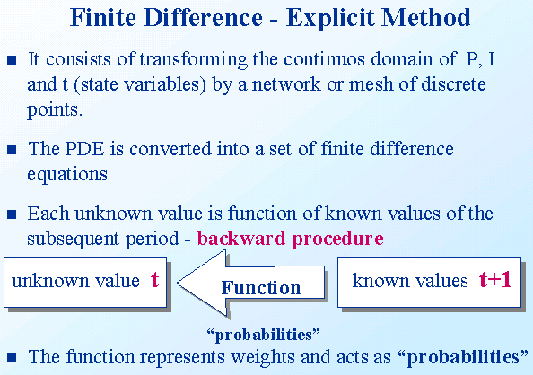
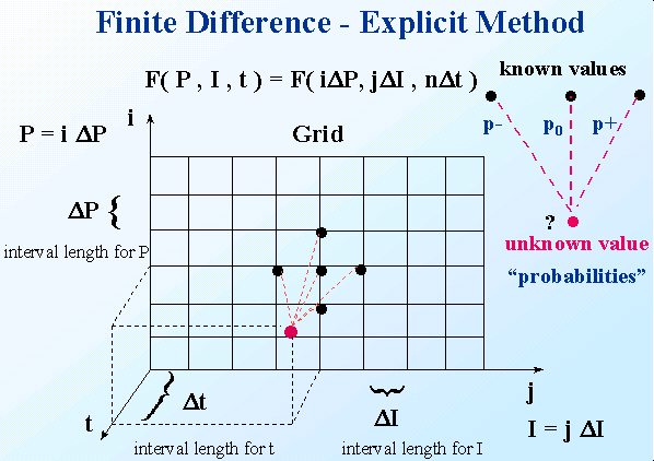
The Finite Difference methods to solve the partial differential equations (PDE) are discussed in more details below, after a short discussion of computational time.
Computational time
It is hard to identify which method is the more efficient. Each one of them has its own characteristics. In general for few state variables, finite difference and lattice methods result in a faster computational time comparing to simulation techniques. However, by increasing the dimensionality of the problem, simulation methods appear to be more efficient and effective. Free boundary problems and optimal stopping problems however are more easily performed and "understood" by finite difference methods.
This section presents a quick overview bout the finite difference method. This method can be used to solve any partial differential equation (PDE) usually found in the financial literature of pricing derivatives in general. It can handle very well free boundary problems and optimal stopping problems.
Let the following linear partial differential equation of second order:
 , (1)
, (1)
where a, b, c, d, e, f and g can be functions of both the independent (x or y), or dependent (u) variable.
It is important to note that the majority of the equations found in the financial literature including exotic options and more sophisticated derivatives, are of parabolic type in one dimention (Black-Scholes equation - one state variable plus time).
However, in Real Option framework we also find eliptic type as well as parabolic type in one or two dimentions (two state variables plus time).
It is important to note that Finite Difference Method are capable of evaluating any type of linear and non-linear Partial Differential Equation as well as Ordinary Differential Equations .
The finite Different Method (FDM) consists of transforming the partial derivatives in difference equations over a small interval.
Assuming that u is function of the independent variables x and y , we can divided the x-y plan in mesh points equal to dx = h e dy = k, as showed bellow :
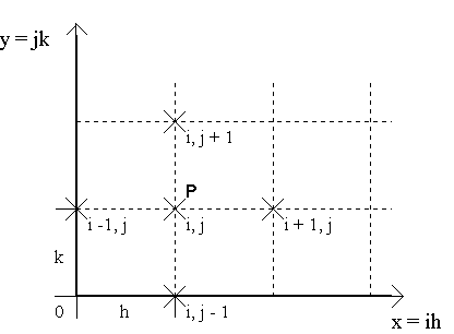
We can evaluate u at point P by :
uP = u(ih,jk) = ui,j
The value of the second derivative at P could also be evaluated by:


The value of the first derivative at P can be evaluated by three approximations:
1) Central difference:


2) Forward difference:


3) Backward difference:


After substituting the derivatives approximations over the PDE, PDE is corverted into a set of finite difference equations that can be solved either by explicit or implicit method.
From now on we will think of the j index as time to expiration (so that j + 1 means more time to expiration, an earlier time instant), and i index as price.
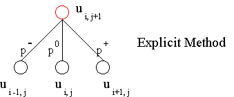
Explicit method allows to evaluate the unknown value today ui,j+1 directly from the subsequent known future values ui-1,j, ui,j and ui+1,j. It can be done because we have proper boundary conditions that always set any values at the termination date. It can be viewd as well as a dynamic programming backward procedure.
Therefore the application of explicit method leads to a difference equation as follow:
![]()
The molecule of a PDE using the explicit method is represented bellow. Unknown value is in red and known values in black:
Implicit method does not allow a directly approach to evaluate the unknown value.
Instead of we found an expression as follows:
![]()
The molecule of a PDE using the implicit method is represented bellow. Unknown values is in red and known value in black:
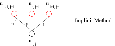
Therefore we have to solve a silmutaneous system of linear equations to evaluate the unknow values.
Supose the parabolic PDE already has been transformed in a set of difference equations. We obtain the following grid where red terms remains to be evaluated.
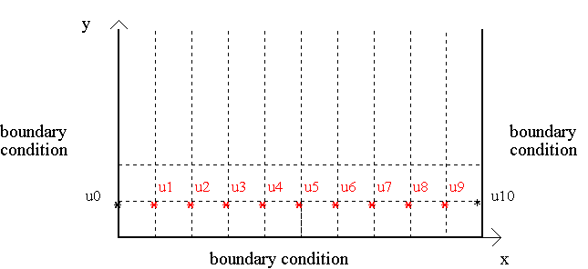
Using the explicit method, the elements u1 - u9 can be evaluated direclty over the subsequent elements, which are the boundary condition 1.
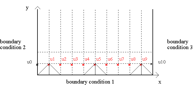
However, if we were using the implicit method we will have a system of 9 simultaneous linear equations, and obtain the 9 unknown values simultaneously.
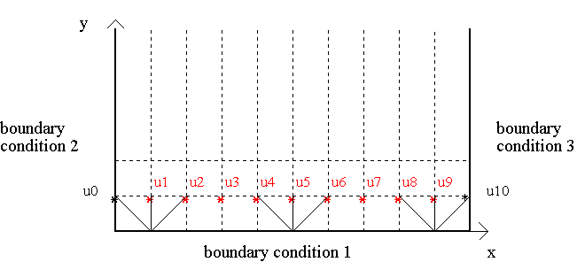
Implicit method is always stable.
Nonetheless, explicit method has to be carefully employed.
For parabolic PDE, after substituting the derivatives by its approximations, it leads to the following difference equation:
![]()
A quick way to guarantee the convergence and stability is set a, b and c > 0 by changing the interval lenght in discretization process.
![]()
![]()