Stochastic Processes and Cycles: Seasonality and Life Cycles Products

Stochastic Processes and Seasonality NEW!

Stochastic Processes and Life Cycles Products

Seasonality can be incorporated into the traditional stochastic processes by changing the drift term.
Tseng & Barz (1998, PSERC Working Paper), use a periodic function m_t for mean reverting processes of commodities prices (both electricity and fuel). Letting p = lnP:

dp = h (p - m_t) + s dz

Where m_t is a cyclical function which p mean-reverts. In the Tseng & Barz paper, interested in short time aspects, m_t was expressed by a table with one m_t value for each hour, a total of 24 values.

A good alternative for the m_t function, are sine/wave functions with maximum at demand peak season.
There are some precautions in this modeling issue. See Dornier and Queruel ( "Caution to the Wind" - Risk, August 2000, Weather Risk Special Report, pp.30-32). They show an example of Chicago's temperature (T), and in order to consider seasonality in the mean-reverting model, the correct mathematical formulation includes an additional term.
The equation for the stochastic variations in the temperature is (with the notation used in this website):

Where: q_t is the mean temperature (which the process reverts) which is a function of time including seasonality, and even a linear trend due to global warming. For example the deterministic time function:

To simulate this process with Dt = 1:

Where e is draws from standard Normal distribution: N(0, 1).

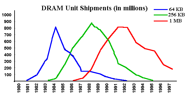
One example is the DRAM memory, computer chips which have increasing demand, following a period of decreasing demand due the introduction of new chips with higher capacity.
The figure below illustrates this case, for 64 KB (kilobytes), 256 KB and 1 MB (megabyte).

This feature is modelled with a regime switching stochastic process.
The following approach most of the time follows the Bollen's paper (1998). See the Bollen's paper: Real Options and Product Life Cycles in his website.

In order to model the demand uncertainty given that there is a regime switching (increasing demand followed by decreasing demand), are used two geometric Brownian motion, being one with positive drift a_i and the other one with negative drift a_d.

The moment of regime switch (shifting from increasing to decreasing) is uncertain, but with increasing probability. Examples:

Let the shifting probability as one function of the demand parameter Y or as a function of the cumulated sales.

Bollen (1998) uses the time normal cumulated distribution F, from the time t₀, to model the regime switch probability.
Example: For a distribution F with expected regime switch of 5 years and with a standard-deviation of 1 year, the demand is decreasing in the year 4 with 2.28% of chance; in the year 6 with 50% chance; and in the year 8 with 97.72% chance.

The goals are:
(a) Calculate the firm value that have options to expansion and contraction, according the demand level;
(b) Choice the optimal initial capacity.
Bollen calculates for the monopoly case, but the extension for the duopoly (or oligopoly) case is not difficult (specify equilibrium, market share).

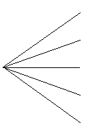
Bollen uses a pentanomial structure (5 branches) to model the uncertainty, with 2 upper branches representing the demand growing and the 2 lower branches representing the demand decreasing.

The following picture shows this pentanomial tree.

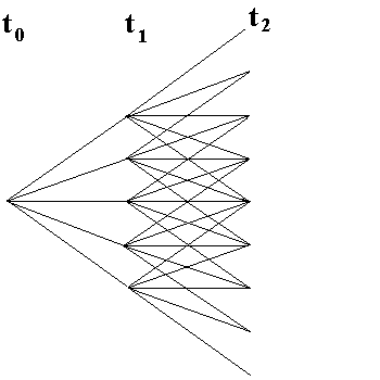
The fifth branch (central branch) is convenient, allowing the recombination in the tree. With 4 branches the tree will not recombine, bringing computational problems.
For 5 branches we get a large economy. For example, for a tree with 500 time-steps, 5 branches instead 4 we get a reduction of 99% in the future quantity of nodes.

The next figure shows the same pentanomial tree, but for two time-steps. Note the recombining tree feature.

This topic is very interesting and some ideas can be used to model seasonality, for example when looking gas natural contracts or projects, which short-term horizon is relevant.

The alternative to the Bollen's lattice framework is a PDE (partial derivative equation) approach.
This is a important topic for future research.