Paddock, Siegel & Smith wrote a series of papers (1983/84/87/88) using options theory to study the value of an offshore lease and the development investment timing.
More realistic models are also possible. For example, the classic model uses the Geometric Brownian Motion for the underlying stochastic variable (the value of the reserve V), whereas one more rigorous but more complex model could be use mean-reverting process with jumps and/or include other options, to allow for other uncertainties sources, etc. One example of these more complex models is presented in another page (petroleum concessions with extendible options, using reversion-jump process to model oil prices).
An American call option is an asset that gives the holder the right (not the obligation) to buy one stock for a fixed exercise price, until a certain date (expiration T).
A simple real option method is to exploit the power of the analogy with
financial American call option on a stock paying a continuosly compound dividend yield.
In this page the analogy is explained and also two main charts are presented and explained.
The main pratical appeal of this analogy with financial option is the simplicity to treat
complex problem of investment under uncertainty.
The analogy financial/real options is particularly interesting when performing sensibility analysis.
The following table presents the American call analogy between financial option and real option, for a general classes of projects (not specific for petroleum projects).
| FINANCIAL OPTION | REAL OPTION (F) |
| Stock or Other Financial Asset | Producing Project (V) |
| Exercise Price of the Option | Investment Cost for the Project (D) |
| Stock Dividend Yield | Cash Flows as Proportion of V (d) |
| Risk-Free Interest Rate | Risk-Free Interest Rate (r) |
| Stock Volatility | Project Value Volatility (or proxy) (s) |
| Time to Expiration of the Option | Time to Expiration of the Investment Opportunity (T) |
There are some differences between the financial and real options, which is necessary to take into consideration. One is the time to expiration: in real options this time is frequently more than one or two years, whereas in financial option case is more typical one or two quarters. In petroleum offshore leases the typical time is 5 to 10 years. The time to expiration is even higher in the case of patents rights.
Other difference is the lag between the starting of investment expenses and the starting of the production, in others words, the time to build the real asset V. This feature can be considered using present value for both investment and asset V. However there are more sophisticated models to capture lag features (exs.: Majd & Pindyck, 1987 and Pindyck, 1993).
Using this analogy, is possible to think one petroleum field development project as an option. In the analogy with petroleum, instead the stock, the underlying asset is the developed reserve value V (which is function of the petroleum prices). The exercise price is the cost of development (D), and the time to expiration (T) is the relinquishment requirement. See details in the deduction of the differential equation of the model.
In this real option model the underlying variable is the
developed reserve market value (project value per barrel).
However, available data and important studies show the high correlation between oil price (P) and
market value of developed reserve (V), so is reasonable to set V as a proportion of P.
The model is valid even if this assumption doesn't hold, but this simplification permits
to use the more familiar oil price P in the charts, as performed in the above chart.
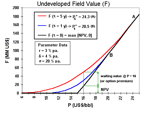
From this model, an option value chart is presented below:

The option chart above shows a black straight line which represents the "now or never" case. The red and blue curves represent the cases of option values for 5 years and 1 year to the expiration of the rights, respectively.
The points A and B, indicated in the chart, are high-contact points, the points where the option curve smooth pasting the straight line from the payoff (the NPV line). At these points, the early exercise are optimal, because the net waiting value (the option premium) is zero.
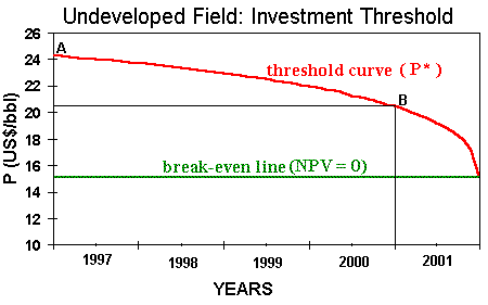
The following chart shows the early exercise line, the threshold curve also known as free-boundary by mathematicians. This line represents the decision rule for the petroleum investment problem.

This chart was drawn with the same data of the other chart (option value). So, also represents the undeveloped oilfield problem, but here faced with the investment decision point of view. The region under the threshold line is the "wait and see" region, whereas above the line is the "immediate investment" region.
Developed Reserve Return = Gain from Production [dividends] + Remaining Reserve Valorization [capital gain]:
![]() ..............(2)
..............(2)
But, the total differential:
![]()
Using the eq.(1):
![]()
Substituing in the eq.(2):
![]() ..............(3)
..............(3)
This is also the eq.(2) in the Dixit & Pindyck, Chapter 12
For a model which the rate of return on the developed reserve follows a geometric Brownian motion:
![]() ...........(4)
. This is also the eq.(3) in the Dixit & Pindyck, Chapter 12
...........(4)
. This is also the eq.(3) in the Dixit & Pindyck, Chapter 12
Substituting eq.(3) in the eq.(4), and "algebring":

![]()
Where the dividend (convenience) yield is:
![]()
The last two equations correspond to the eqs.(4) and (5) in the Dixit & Pindyck, Chapter 12
Itô Lemma for F (V, t ) is:
![]()
where the subscripts denotes partial derivatives
Squaring the stochastic equation (eq.5), and for dt infinitesimally small, terms with
dt of order > 1 can be ignored (e.g. dt.dz is of order dt3/2 and can be ignored) :
![]()
![]()
The risk-free portfolio values:
![]()
The quantity of stocks n to built a risk-free portfolio is the derivative of the option (named "delta" in financial market), because makes the random term (dz), of the return equation, equal to zero.
The portfolio return per barrel is:
![]()
But the portfolio return per barrel is also:
Obs: also is OK the thinking with the dividend yield:
![]()
![]()
Equaling with eq.(10) and substituting dF in the eq.(9):
![]()
Simplifying (note that the dt terms are ruled out):

Finally, substituing the dividend yield (eq.6), result in the partial (t, V) differential equation:
Which is also presented in Dixit & Pindyck book.