In this webpage is presented the model for petroleum concessions (real options) with extendible maturities.
This section has the following features:
See or download the paper "Petroleum Concessions with Extendible Options Using Mean Reversion with Jumps to Model Oil Prices":
Download a slightly different (version of late 1998) paper version, in the SSRN database, by clicking here.
Petroleum firms acting in exploration and production (E&P) routinely need to evaluate concessions and to decide the investment timing for its project portfolio. In some countries, the exploration concession has features such as the possibility of extension of the exploratory period. The holder of a petroleum exploration concession has an investment option until the expiration date fixed by the governmental agency, and these rights can be extended by additional cost. The additional costs can be some fee (extra-tax) to governmental agency and/or additional exploratory/appraisal investment.
The value of these rights and the optimal investment timing thresholds are calculated by solving a stochastic optimal control problem of an American call option with extendible maturities, using the dynamic programming framework. The thresholds for both the optimal extension of the option and the immediate development investment are presented and discussed.
The uncertainty of the oil prices is modeled as a mix jump-diffusion process. Normal information generates continuous mean-reverting process for oil prices, whereas random abnormal information generates discrete jumps of random size. We adapt the Merton (1976) jump-diffusion idea to the oil prices case. Normal information means both marginal interaction between production and demand (inventory levels is an indicator) and depletion versus new reserves discoveries (the ratio of reserves/production is an indicator).
Abnormal information means very important news, causing in a short time interval, a large variation (jumps) in the prices. These jumps, which has been observed sometimes in oil prices history, are modelled with a Poisson process.
The paper's new contributions are two: the framework of options with extendible maturities for real assets and the utilization of a mixed stochastic process (mean-reversion with jumps) to model the petroleum prices which, despite of its economic logic, has not been used before in petroleum economic literature. Comparisons are performed with the popular geometric Brownian process for both the concession option value and the optimal investment timing policy. The role of the convenience yield is also discussed for both stochastic processes, which has an important impact in the optimal development investment threshold. Analysis of alternative timing policies for the petroleum sector is presented, and also the comparative statics for the main parameters of the model.
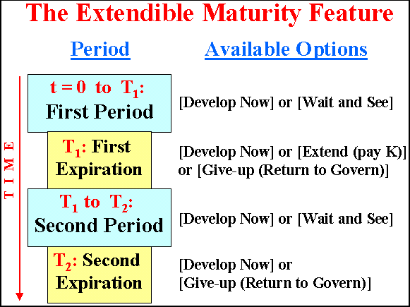
This option allow the holder of the exploration concession to extend the deadline of the investment in the oilfield development by paying a fee K (taxes and/or additional exploratory/appraisal costs). So there are two expirations for this extendible option.
The following picture illustrates the extendible option feature in petroleum Exploration and Production (E&P):
In a more recent version of ANP (Brazilian National Petroleum Agency)
contract, appears the possibility of a third exploratory period.
So there are three expirations in exploratory phase.
Of course the model is analog to the presented here, and no affect the
main insights drawn with two expirations model. Anyway, the upgrade of
this model allowing for three periods is planned for a near future.
The following slide illustrates the Exploration and Production (E&P) Process and the focus of our model:
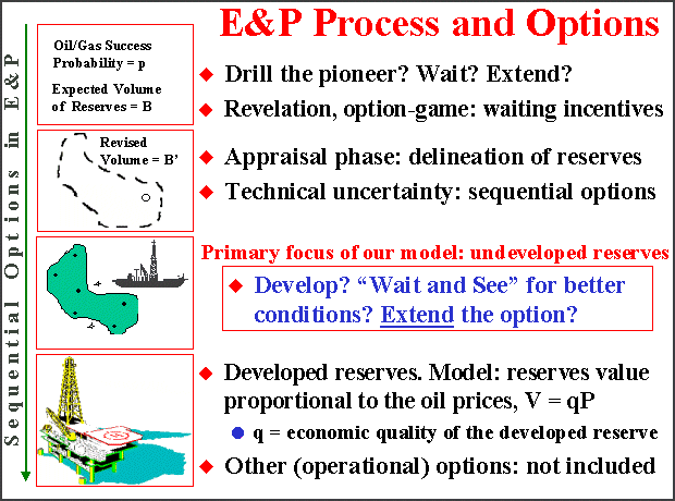
The application of the model is much more general in the sense that can
be used for investment decisions on the appraisal phase, for wildcat
drilling decision and even for bonus calculus in the bidding process of a
petroleum concession.
This is due to calculus processing that is done backwards,
so we need to estimate the development options values to estimate the
prospect value.
The solution of the model is presented for both stochastic processes, the traditional geometric Brownian motion and the new and more general stochastic process of mean-reversion with jumps to model the oil prices uncertainty.
This model is detailed in the paper of Marco A.G. Dias & Katia M.C. Rocha (1999).
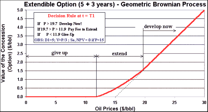
The payoff at the first expiration (T1) considers the
special feature of the option to extend the concession rights.
The payoff at the first expiration for the geometric Brownian case, which
has the feature to extend for more three years is presented below:
For the model of jump-reversion, the stochastic equation is:


For this compensated Poisson reversion, the drift or the expected value for the capital gain E[dP/P] is given by:

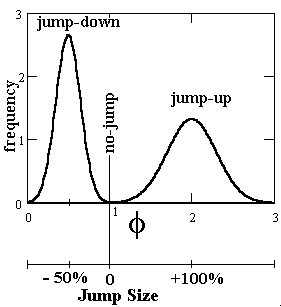
The jump-size is random and is represented with a two truncated normal
distributions, one normal for the jump-up and the other for the jump-down.
There are the same chances for a jump be up or down.
The figure below illustrates the jump size distribution:
Using the dynamic programming with an exogenous discount rate r a la Dixit & Pindyck (1994), in order to maximize the value of the option opportunity under uncertainty, the Bellman-dynamic programming equations are:
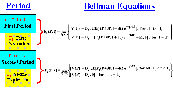
Using the dynamic programming with an exogenous discount rate r, can be demonstrated that the value of the one undeveloped reserve (option) F in function of the petroleum price follows the partial differential equation below:

The contingent claims version of the model (considers the jump risk non-systematic) is very close of the dynamic programming version, changing in the above equation only in the second term of left side and in the right side, as showed below:
In red is highlighted the parts of the equation that change for the contingent claims.
Note that even for contingent claims is necessary to estimate r, in this case because the value of d: For mean-reversion models like our, the equation for d is given by
d = r - a = r - h(
![]() -
P)
-
P)
Why this not occurs for geometric Brownian motion (GBM) models? Because
in GBM the dividend yield/convenience yield d
is assumed constant.
In contrast, here (models with mean-reversion) the drift is specified and
so the risk-adjusted discount rate.
More: the convenience yield is also function of P. In some cases it can
become even negative for low values of P. For d
negative, the [American] real option will not be exercised before the
expiration (this is a very known result of American options early exercise
feature).
This feature is showed in some graphs, and explain thresholds
discontinuities.
The boundary conditions, including smooth pasting optimal conditions, are presented below (remember that NPV = V - D = q P - D):
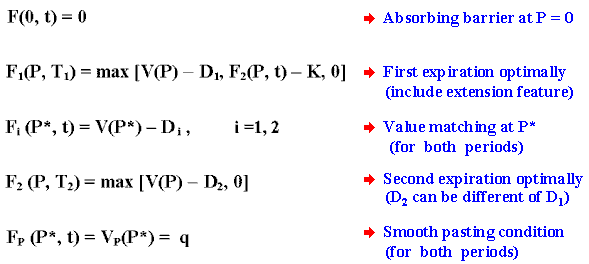
In order to solve the PDE, we used a finite differences method in
explicit form, and a C++ software was developed with an interactive
interface.
See the software in The Real Options Software
Webpage, computer programming languages section.
The main results of our model in terms of options values, thresholds for immediate development at both t = 0 (current instant) and t = T1, and thresholds for extension (at t = T1) is displayed in the table below.
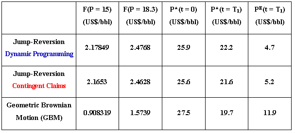
The results using dynamic programming and contingent claims for the same
jump-reversion process are very close, whereas very different of the
geometric Brownian case.
We adopt for contingent claims the same risk-adjusted discount rate
r = 10% p.a., and a risk-free interest rate r
= 5% p.a.
For GBM, we adopt the same risk-free interest rate and a convenience yield
d = 5% p.a.
For all the jump-reversion base case parameters, see a table clicking here or go to the next page on extendible option model.
The options charts for the two periods and two expirations are displayed
below.
The charts are for the mean-reversion with jumps base case.
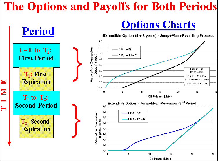
The first expiration payoff exhibits the extendible region for
intermediate oil prices. In the second expiration the payoff is the
traditional American call payoff, without new extensions.
The picture also shows the option values at the beginning of each period,
that is, at t = 0 and t = 5.1 years.
The following chart presents a threshold comparison between the mean-reversion with jump process and the popular geometric Brownian motion (GBM) process.
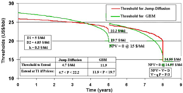
The threshold line for jump-reversion process has lower variation with
time for most of time.
This low sensitivity of the threshold suggest that a longer timing policy
will not incentive much the investment delay.
Consider the following values for different timing policies given in the
table below.

For some alternative timing policies, are presented the option value
(proxy of a bonus bid) and the thresholds values (give an idea on
investment optimal delay). See that the timing policy effect is more
important for option values. If a project is good enough
(deep-in-the-money) a higher timing policy in general will not delay the
investment, whereas if a project is not good enough, a shorter timing
policy in general will not incentive immediate investment.
The only significant benefit for the govern to adopt a shorter timing is
a earlier "now-or-never" situation, for positive NPV projects
but not enough to shot an earlier option exercise.
A higher timing policy however means more significant option value. So
this can be advantageous. The paper shows that by increasing timing policy
(the total expiration of the option, T1 + T2) the effect on option values
are more significant than the threshold variation.
In addition, other reasons points a higher concession value for higher
timing policies (until ~12 years), so the National Petroleum Agency will
get higher bonus bid (and attract more companies) with more generous
timing policy.
This conclusion was mentioned by the notable economist, Deputy and
former Finance Ministry Antonio Delfim Netto in a Brazilian top newspaper,
"Folha de São Paulo", in April 14, 1999.
See the Delfim Netto article by
clicking here (in Portuguese).
This article is also reproduced in
Starmedia website (in Portuguese).
See also the
PUC-Rio's internal newspaper article ("Jornal da PUC", June 1999) about this success in petroleum sector debate (in Portuguese, with photo).
Other feature in the threshold chart above is that near of the second
expiration the threshold curve is well above the break-even price (price
so that NPV = 0), mainly because the convenience yield is negative in this
lower prices region.
For negative convenience yield the earlier exercise is never optimal, this
is a known result from the American call literature. At the expiration,
there is a "now or never" opportunity and in this model (without
operational options), the NPV rule is valid. This explain the sudden drop
of the threshold line at the second expiration.
The following chart shows an interesting feature of the extendible option problem.
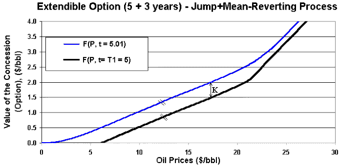
The option curve immediately after the first expiration (just after
paying the fee K) and the payoff curve at T1 in the region
that is optimal to extend (between ~6 to ~22 $/bbl), are two parallel
option curves.
The distance between these parallel curves is just the extension fee K.
Boundary condition explains parallel distance of K in that interval.
The chart uses K = 0.5 $/bbl (instead base case K = 0.3) in order to
highlight the effect.
In this website are presented the general guidelines of the model and several comparative statics that was not included in the paper (due space restrictions).
![]() Click
here to see a webpage with the sensitivity analysis of this model.
There are many charts showing the variations of the real option value and
the thresholds with several parameters.
Click
here to see a webpage with the sensitivity analysis of this model.
There are many charts showing the variations of the real option value and
the thresholds with several parameters.
The main objective of this page is to complement the paper and even to
make some upgrades and new analysis in future.