Economic Quality of a Reserve

Last Update: June 2003.

In this webpage is presented the concept of economic quality of a reserve, including an application of this concept for mutually exclusive project selection under uncertainty, and some FAQs. The topics are presented below:

Introduction to Economic Quality of a Reserve

Application: Selection of Mutually Exclusive Alternatives under Uncertainty

Some FAQs on the Economic Quality of a Developed Reserve

This concept was presented at the Real Options Workshop, in May 1998, Stavanger, Norway. I take some slides from the my workshop presentation, but with some intermediates comments.

The undeveloped reserve value (F) is the real option value to develop the reserve. A developed reserve is a producing (or ready to produce) asset with value V. We can think V in unitary value ($/bbl, where bbl = barrel) or as the value of the whole developed reserve (in million $).

The economic quality of V depends of the nature (rock/fluids properties), but also depends of the location (if onshore or offshore; shallow or deepwaters; fiscal/tax regime of the host-country; etc.) and of the development project (depending of the capital intensity alternative, petroleum can be extracted faster or slower; with high or low operational costs; etc.).

The concept of economic quality of reserves catches these features. It can be estimated using the traditional discounted cash flow or more sophisticated approaches (e.g., including abandonment option).

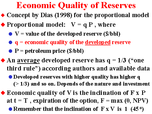
In the proportional model (reserve value proportional to oil prices) also named The Business Model, is easy to work with both charts for the option value, F x V and F x P (if you have one chart, is easy to get the other one). However, the concept of economic quality of a reserve works with the F x P chart, because it is the payoff line inclination.

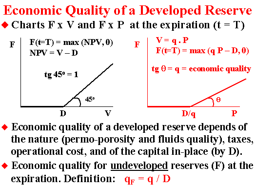
An alternative definition for q_F, the economic quality of the undeveloped reserve, could be:
If t = T, q_F = Max[NPV, 0]/P; and
If t < T, q_F = F/P
With this alternative q_F definition, by multiplying q_F times P, we get the value of one barrel of undeveloped reserve (F). This is similar with the case of q itself: q times P gives V, the value of the developed reserve.

Application: Selection of Mutually Exclusive Alternatives under Uncertainty

The choice of the better alternative of development is one important step that is performed through technical-economic feasibility studies, where several alternatives that imply in several different economic quality for the resulting developed reserve.
The concept of economic quality permits an easy comparison of alternatives with different investments, operational costs and revenues, considering the timing to develop and the uncertainty on oil prices.

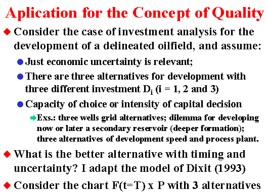
The alternatives have different investment costs. Higher investment alternatives have benefit of faster production (more wells and/or higher processing facilities capacity) and/or lower operational costs.
What is the optimal capital intensity under uncertainty?

This model is adapted from: Dixit, A.K. (1993): "Choosing Among Alternative Discrete Investment Projects Under Uncertainty". Economic Letters, vol.41, 1993, pp.265-288. However, I consider finite-lived real options, whereas Prof. Dixit considered perpetual options.
Recently, Décamps & Mariotti & Villeneuve (2003): "Irreversible Investment in Alternative Projects", Working Paper from Université de Toulouse and London School of Economics and Political Science, give important and rigorous additional contributions to this model, which will be pointed out soon in this page.

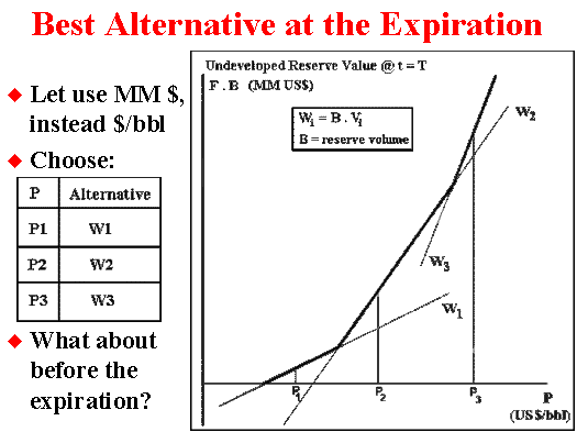
The higher inclination (or higher quality q) alternative 3 has the higher investment. Of course alternatives with higher investment but with lower quality (inclination) is dominated by higher quality alternatives and can be eliminated.

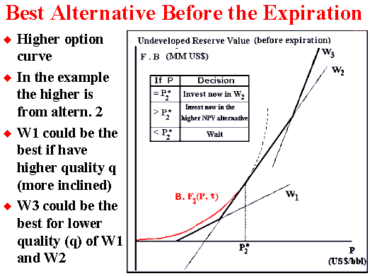
It is easy to get the curves for the option alternatives with spreadsheets like Timing. To compare, superpose the option curves and look for the higher one. With this practical approach we can see some special cases not addressed before by Dixit (1993). Even being an approximation (see below why), the numerical error on the value of the option is very small so that it possible to see that in most cases there is an intermediate waiting region between the exercise of alternatives 2 and 3. So that for P > P*₂, we can see a region that the option value of waiting (F₃) is higher than both NPV₂ and NPV₃.
Motived with this somelike surprising experimental early result, in 2000 were started two projects between PUC and Petrobras - from the Pravap-14 research projects portfolio, which confirmed this hypothesis. One Pravap-14 project was a more flexible and general determination of the optimal rules regions by using genetic algorithms (developed with Electrical Engineering Department). The other Pravap-14 project was more rigorous (but specific for simpler cases) using the traditional differential equation approach (developed with Industrial Engineering Department). Both used finite-lived options. In year 2002 we started the second phase of both projects, adding other realistic details with more complex issues.
By using a C++ PRAVAP-14 software developed at Industrial Engineering Department (PUC-Rio), it is possible to get the following thresholds chart showed below (and presented at MIT Seminar on Real Options, May 2002).

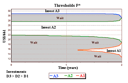
Working independently and with perpetual options, Décamps & Mariotti & Villeneuve (2003) proved mathematically that the waiting region around the point of indifference between NPV₂ and NPV₃ always occurs (non-empty region) if sometimes is optimal to invest in alternative 2. They showed that if "investment in the smaller scale project is sometimes optimal, ... the optimal investment region is dichotomous.". In their proposition 3.2, they show that the indifference point where NPV₂ = NPV₃ does not belong to the exercise region. They proved with help of the sophisticated concept of local time for the continuous semimartingale P applied at this indifference point. Before this paper, I was thinking that the Dixit's (1993) claim even not being typical could be possible. But they proved that it cannot be possible.

Probably the conclusion from Décamps & Mariotti & Villeneuve (2003) is even more general, being also true for finite-lived options except at the expiration.
I thank to Professor Thomas Mariotti for letting me know about this paper and for the nice discussion.
With this new insight in mind, we can correct the Dixit's option value chart by setting a case that always occurs in the figure below (analogous to Figure 1 from Décamps & Mariotti & Villeneuve, 2003):

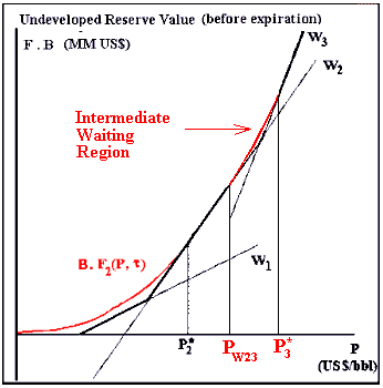
In the above figure, the option curve (red line) in the superior part of this figure (between P_W23 and P*₃) is the intermediate waiting region. Décamps & Mariotti & Villeneuve (2003) showed that this region always exists (if sometimes is optimal exercise alternative 2, as occurs in the figure).
Numerically the error can be small if exercising the option (higher NPV as suggested by Dixit in 1993) rather than waiting in this intermediate optimal waiting region. So, even not being correct, the error using the Dixit's insight can be small in practice. However, the size of the waiting interval (between P_W23 and P*₃) can be a large range.

But in addition to be optimal the "waiting and see" policy at this region, the option curve value (let us call B . F₃) can also indicate something about an optimal project scale. If P belongs to this intermediate waiting region, the optimal scale project for an immediate investment exercise must have a quality q* equal to the derivative of this option value, that is, q*(P) is equal to derivative of B . F₃ in relation to P. This conclusion is derived from the smooth-pasting property at the optimal option exercise. This project does not exist in the figure above, but the optimal scale in this case is an intermediate scale between the alternatives 2 and 3. So, there is an interesting practical link between the concept of quality q and the smooth-pasting property for the optimal scale.

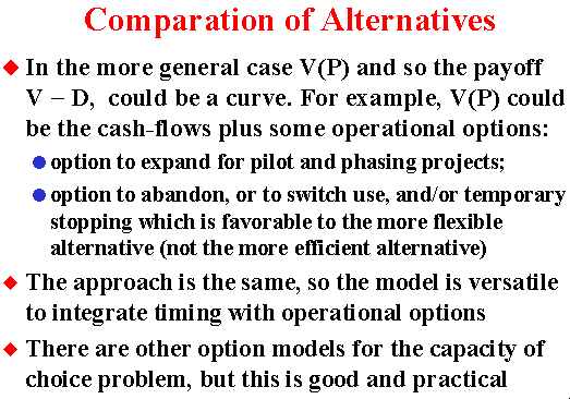
The approach using the concept of economic quality of a reserve can be extended to more complex situations. See the slide below.

For the fiscal regime of concessions (USA, UK, Brazil, and others), the linear equation for the NPV with the oil prices is at least a very good approximation. For the fiscal regime of production sharing (used for example in Africa), the same is not true (for the production sharing case including the NPV x P chart, click here).

If the underlying asset V is a linear function of P, that is, V = a P + b, and if the constant a > 0, we can say that V and P are perfectly positively correlated (coefficient of correlation between V and P is equal + 1). See the proof for example in the DeGroot & Schervish's text, p.218 (Probability and Statistics, Addison-Wesley, 3rd Edition, 2002).

The figure below presents two different linear equations for the NPV equation (NPV = V - D), using different definitions for the value of the underlying asset (the reserve value V). One is named "Business Model" and the other one is named "Rigid Cash Flow Model".

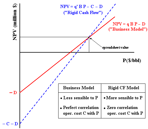
In order to understand the "Business Model", think about the market value of one barrel of reserve v (that is, v is the price of the barrel of reserve). If this reserve price v is directly related with the long-run oil prices, let be q the factor of proportionality so that v = q P. For developed reserve transactions, as higher is the price per barrel of a specific reserve, as higher is the economic quality for that reserve. For a fixed reserve volume and fixed oil price, as higher is the factor q as higher is the value of this reserve.
By using this insight, the value of a reserve V is the price of the barrel of reserve v times the size of this reserve B, that is, V = v B. The equation for the developed reserve value V is:

V = q B P.

This is the easiest way to work with the three most relevant variables to access the value of a developed reserve, using business thinking, which is very adequate for market valuation. The value q can be assessed either by market transactions in markets like USA (see Adelman & Koehn & Silva, 1989; and Adelman & Watkins, 1996) or by using the discounted cash flow approach.
In the first case, is necessary to consider the appropriate discounting effect on q in order to put in present value the reserve value V (see also the FAQ 3 below in this page). Note that q is the only parameter to consider the discounting effect in the equation of V.
In the second case, consider the spreadsheet NPV estimate for a certain (average) oil price. In a chart NPV x P this base-case NPV estimative, is one point of our straight line, the other one is defined by NPV(P=0) = - D. The figure above presents the link between this chart and the equation for the "Business Model".

The Rigid Cash Flow Model is given by the equation:

V = q' B P - C.

Where C is a kind of fixed operational cost in present value. In the Rigid Cash Flow Model the quality of reserve is given by q' and is higher when compared with the quality from the business model.

In comparison with the "Business Model", the model named "Rigid Cash Flow" is more sensible to the oil prices. In general this means higher real options value F(P) for the "Rigid Cash Flow Model". In this aspect the "Business Model" is more conservative.

The "Rigid Cash Flow Model" assumes no correlation between the operational cost (C) and the oil price (P). In reality, microeconomic logic points that a positive correlation is expected to occur between C and P because the main costs are industry-specific. For example, wells maintenance are done by specific rigs, oil transport demands tankers, many specific petroleum services, etc. The microeconomic logic of correlation means that higher oil prices tends to increase the demand for specific petroleum services, increasing the operational cost C, and vice versa.
The truth on the correlation lies between the "Business Model" (perfect positive correlation) and the "Rigid Cash Flow Model" (zero correlation). However, an intermediate model means to assume the operational cost C as stochastic, introducing some additional complexity to the model.

More about these payoff models, the specific spreadsheets Timing Version Business Model and Timing Version Rigid Cash Flow Model, non-linear models, proofs, etc., see the webpage Linear and Nonlinear Models for the Underlying Asset V(P) and the NPV Equation.

I list here some FAQs (frequently asked questions) and practical issues. Let us go to the first question:

1) Is this linear model (V linear in P) reasonable?

The easiest way to apply the concept of economic quality of a reserve is by using the linear model because the quality q is constant.
However, the quality concept doesn't depend on the linear model.
If V is a non-linear function of P, the quality q is a function of P equal the derivative of V(P), that is, q(P) = V/ P.

The assumption of linearity has been considered reasonable in the real options literature, see for example Dixit & Pindyck (1994, chapter 12, section 1) and Paddock, Siegel & Smith (1988).

Schwartz ("The Stochastic Behavior of Commodity Prices: Implications for Valuation and Hedging", Journal of Finance, vol.52, number 3, July 1997, see p.971) results give us another important argument, using very different stochastic models that driven heavily on futures markets insights (the two and three-factor models).
These models imply an underlying project value that is linear with the spot price (Schwartz, 1997, Fig.13), the inclination of his two or three factor NPV is exactly our economic quality q.

Schwartz (1997) two factors model presents the following equation for the forward (or futures, the interest rate is non-stochastic here) prices F:

F(P, d, t) = S exp{- d [(1 - e^{- h t} )/ h] + A(t) }

Where A(t) depends of the time and the parameters process, but not depend neither on the spot price S nor on the convenience yield d.
h is the reversion speed of the stochastic convenience yield.
Note that forward (futures) prices F is a linear function of the spot price S.

Now Schwartz calculates the NPV per unit of product (his equation 49) as a function of the present value of the commodity produced at the instant t, which is the discounted value from the forward prices, less the present value of the operation costs (he assumes known and not a function of S) less the unitary investment cost (which is not a function of S).
Using futures equation for commodities prices like the presented above, Schwartz present the NPV equation for a project, which implies in the linear relation NPV with spot prices for two factors model, as well as for three factors models and for geometric Brownian motion (his Fig.13).

For his two factors model, but for time varying production Q(t), following a typical decline in petroleum case, the economic quality of a developed reserve is:

q = Q(t) exp{- d [(1 - e^{- h t} )/ h] - r t + A(t) }

In his example the production last for ten years, using annual discretization for NPV calculus. A(t) is as before.

As pointed out by Schwartz (1997, Fig.13), for pure mean-reversion models the NPV is not a linear function (even being a good approximation in many cases).

2) A practical issue: How to calculate the economic quality of a developed reserve if I have the spreadsheet with the traditional discounted cash flow?

Everybody has this kind of spreadsheet, so you get the NPV (net present value), the break-even price (unitary cost of production, UCP, the price which the NPV is zero), and the after-tax investment (present value) D.
Lets work with unitary value (per barrels of oil equivalent, BOE). So, think unitary (per BOE) values for NPV and D.

The most common practical problem is related the consequences of non-linearity of the function V(P) for most spreadsheets results, even when linearity is a very good approximation.
The figure below shows, for a non-linear V(P), two points (A and B) which has two differents economic qualities. One point (B) is the current valuation (with current petroleum prices) resulting in the NPV displayed. The other point (A) is the point which NPV is zero. This is the break-even or unitary production cost (UPC).
The inclination q is different depending what point is choosen for evaluate q.

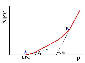
So, to be consistent with the spreadsheet discount cash flow analysis for the current price and the associated NPV, this means you get another UPC (different of the spreadsheet). If you is consistent with UCP, this means that the NPV for the same price level will be different of the DCF spreadsheet. What the better point to estimate q?
I prefer to evaluate q in the current situation (instead in the UPC point), because the estimative of cash flows generally are more reliable for the base-case.

The method relying on the actual NPV and associated current price level, that is, relying on the relation q = V/P(t=0) is presented below. The steps to calculate q and V are:
1) Calculate D, the unitary (per BOE) present value of investment cash flow, net of fiscal benefit (after-tax);
2) Calculate V = NPV + D, where NPV is the net present value per BOE; and
3) Calculate q = V/P(t=0); where P(t=0) is the current petroleum price used (or an equivalent price for a mix of products like gas + oil).

The method relying on the break-even value (UPC), that is, relying on the relation q = D/UPC, is presented below. The steps to calculate q and V are:
1) Calculate D, the unitary (per BOE) present value of investment cash flow, net of fiscal benefit (after-tax);
2) Calculate q = D/UPC, where UPC = unitary production cost or break-even cost; and
3) Calculate V = NPV + D

3) Is there some effect of discount rate on the value of the economic quality of developed reserve?

Yes. The discount rate (r) affect the economic quality of the reserve (q).
The two main discount rate effects on q are:

• The whole value of q is affected because q reflects the operational cash-flow in present value terms. So, companies with higher capital cost has less valuable reserves in economic terms than companies with lower capital cost. The implication for dealing with reserves (selling and buying) is evident.
• The value of q in the equation (values per barrel) NPV = q.P - D, means that both q and D are discounted to some initial date. So, if you are using q to estimate the immediate investment to develop the field and this takes three years (time to build) to start-up the production, the value of q will be reduced by a discount factor for these three years. Hence, the value of q for producing oil assets (in a farm-out business) is higher than the value of q used for investment analysis, due the discount factor of three years.

In the last case, when analysing exploratory prospects (drill or not the wildcat), the discount factor effect makes the value of q even lower than the one used in development applications.

In short, is not possible to compare directly the 1/3 rule (average q = 33.3% for USA developed reserves) with the values used in both applications, development investment and exploratory investment, due the discount rate effect.
For example: For a discount rate of 10% p.a., an offshore reserve if is producing has a q = 33.3%; but if it is an economic study of development investment that takes time to build of three years, for the same reserve q = 24.7%; and if it is an exploratory investment study so that the first-oil will come in 5 years, value of the q drops to 20.2%.