In this webpage are presented both linear and nonlinear equations for
the value of the underlying asset (V) as function of the commodity price
P. Consequently, are developed equations for the net present value
equation NPV(P) = V(P) - D for the
project development, considering a development investment D.
OBS: Sometimes I use the notation "D" for the development
investment, and in other situations I use the more general notation "I"
for the investment. In both cases consider "investment" as the
present value of the investment (not the nominal one).
This webpage topics are:
![]() Linear
Models for the NPV Equation
Linear
Models for the NPV Equation
![]() Nonlinear
Models for the NPV Equation
Nonlinear
Models for the NPV Equation
OBS: Because I use the tag "Font Symbol" for the "Greeks"
letters, it is recommendable to use the browser Internet Explorer or
Netscape until version 4.x. Unfortunately, Netscape versions 6.x and 7.x
don't support "Font Symbol" for the "Greeks" letters
anymore (I think this is a big drawback for the new versions of Netscape -
a negative evolution).
If you is looking the letter "s"
as "s" instead of the Greek letter "sigma", your
browser doesn't support "Font Symbol".
In this case, the reader can download the pdf version of this page,
payoff_model.pdf with 488 KB (pdf quality
is inferior to the browser printing one)
This recommendation is also valid for many pages in this website that work with equations.
Initially, consider only the optimal timing to exercise the option to develop a project. The payoff from exercising the option to develop the project, is the net present value (NPV). The NPV is equal to the present value of revenues net of operational costs and taxes (V) less the present value of the investment cost I net of fiscal benefits (NPV = V - I). For while, we are not including operational options, that is, options after the development (option to expand, option to stop temporally, option to abandon).
In some cases, we can adopt a simple proceeding such as the one
suggested by Copeland & Antikarov's textbook (2001), considering only
a geometric Brownian motion for V with volatility estimated from the
distribution of present values of V at t = 1. This distribution results
from a combination of uncertainties using a Monte Carlo simulation.
However, in some cases this procedure is not adequate because we want to
make explicit some key variables along the model. One example is the case
of value of information, where nature of the
process of information revelation of technical uncertainties is totally
different of a Brownian motion, so that it is not possible to combine
these uncertainties to get a "total volatility" for V.
Specially for these richer cases, we need to work with payoff (NPV)
functions making explicit some key variables like the price of product P, the
reserve volume B, the reserve quality q, the operational costs OC, etc.
In these more complex problems we need to work with Monte Carlo
simulation to combine technical and economic uncertainties. A
practical challenge in petroleum projects is how to model the NPV function
when performing a Monte Carlo simulation of the key factors with technical
and economic uncertainties. There are at least three alternatives
to consider both technical and economic uncertainties into the NPV
function.
First using a model as simple as possible but considering the main
uncertainties, which are parameterized from the DCF (discounted cash flow)
model or drawn from a business vision of the project. This kind of model
and its variations will be detailed later.
The second alternative is by working directly with the cash-flows, for
example an integral with revenues and costs explicitly written as function
of variables with uncertainty . This can be done also by putting formulas
and correlation among cells in the spreadsheet linked to the sources of
uncertainties, because the Monte Carlo simulation needs to change every
cell in the appropriated way. Although this is possible, the formulas can
be complex to link the uncertainties on the reserve size and productivity
of wells, complicating the interpretation and with a much higher
computational cost than the first alternative. This second way was used in
the PUC-Petrobras research project to model an option to expand the
production through new wells. This case was easier than the general
case because the technical parameter was set at well level outcome.
The third alternative for a Monte Carlo simulation of the NPV function is
by using more complex models and tools in tandem. The technical
uncertainties are introduced into the reservoir simulator software,
generating the distribution of production profile with its associated
values for V and D (and so the NPV = V - D) in
the NPV spreadsheet. The problem is that the reservoir simulator is called
for every sample used in the Monte Carlo simulation, and the reservoir
simulator (that solves a system of partial differential equations)
is not fast enough, so that the computation is very slow. In the future,
it will become the preferable one because uses the revelation
distributions in a more realistic way.
Since the NPV is just a linear function of the expected cash-flows, it
is natural to consider models which the NPV is a linear function of the
price of the product (e.g., oil price P), because cash-flows in general
are also linear function of P.
Linear models for the variation of V (or the NPV) with the output prices P
are the most important models inside and outside the petroleum industry,
due to its practical relevance.
In petroleum projects, for the fiscal regime of concessions (USA, UK, Brazil, and others), the linear equation for the NPV with the oil prices is at least a very good approximation. For the fiscal regime of production sharing (used for example in Africa), the same is not true ( see nonlinear NPV topic).
If the underlying asset V is a linear function of P, that is, V = a P + b, and if the constant a > 0, we can say that V and P are perfectly positively correlated (coefficient of correlation between V and P is equal + 1). See the proof for example in the DeGroot & Schervish's text, p.218 (Probability and Statistics, Addison-Wesley, 3rd Edition, 2002).
The development below uses a petroleum development project as guide.
However, similar reasoning applies in many other industries.
Assume that D = investment cost to develop the petroleum project
with volume of B barrels of reserve. This project has a random
benefit V. This benefit in this petroleum case is the value of
the developed reserve. A factor q or q' (depending of
the model) will be named economic quality of the reserve for the
petroleum case (because as higher is q, as higher is the developed reserve
value V, for details on q click here).
The figure below presents two different linear equations for the NPV equation (NPV = V - D), using different definitions for the value of the underlying asset (the reserve value V). One is named "Business Model" and the other one is named "Rigid Cash Flow Model".
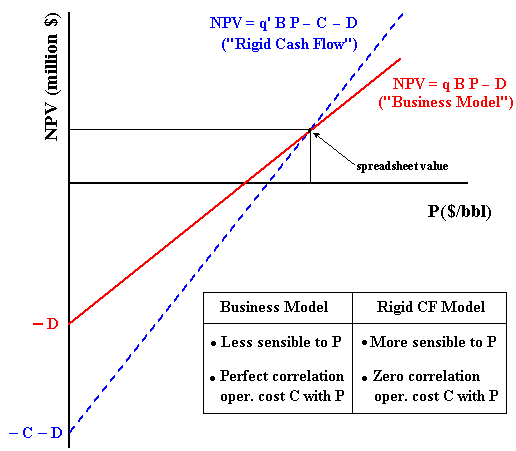
In comparison with the "Business Model", the model named "Rigid
Cash Flow" is more sensible to the oil prices. The intuition says
that this means higher real options value F(P) for the "Rigid Cash
Flow Model". In this aspect the "Business Model" is more
conservative about the value of the investment timing option. This
intuition will be confirmed with the numerical results of an example drawn
from the Timing (Excel spreadsheet) versions for both models.
In addition, for lower oil prices the option to shut-down could
have a non-negligible value (reducing the losses predicted in the "Rigid
Cash Flow Model" chart).
The "Business Model" assumes that the operational cost is proportional
to the price P, so that there is a perfect positive correlation between
operational cost and price. The "Rigid Cash Flow Model" assumes
zero correlation between the operational cost (C) and the oil
price (P). In reality, microeconomics logic points that a positive
correlation is expected to occur between C and P because the main costs
are industry-specific. For example, wells maintenance are done by specific
rigs, oil transport demands tankers, and many others petroleum services
are industry-specific. The microeconomics logic of correlation means that
higher oil prices tends to increase the demand for specific petroleum
services, increasing the operational cost C, and vice versa.
The truth on the correlation lies between the "Business Model"
(perfect positive correlation) and the "Rigid Cash Flow Model"
(zero correlation). However, an intermediate model means to assume the
operational cost C as stochastic, introducing some additional complexity
to the model.
In the next sub-topics both models are detailed and some results and proofs are presented. Return to figure above when necessary to understand better the models.
In order to understand the "Business Model", think about the
market value of one barrel of developed reserve v (that
is, v is the price of the barrel of developed reserve). If this reserve
price v is directly related with the long-run oil prices, let be q the
factor of proportionality so that v = q P. For developed reserve
transactions, as higher is the price per barrel of a specific reserve, as
higher is the economic quality for that reserve. For a fixed reserve
volume and fixed oil price, as higher is the factor q as higher is the
value of this reserve.
By using this insight, the value of a reserve V is the price of the barrel
of reserve v times the size of this reserve B, that is, V = v B.
The equation for the developed reserve value V is:
V = q B P.
This is the easiest way to work with the three most
relevant variables to access the value of a developed reserve, using
business thinking, which is very adequate for market valuation. The value
q can be assessed either by market transactions in markets like USA (see
Adelman & Koehn & Silva, 1989; and Adelman & Watkins, 1996) or
by using the discounted cash flow approach.
In the first case, is necessary to consider the appropriate discounting
effect on q in order to put in present value the reserve value V. Note
that q is the only parameter to consider the discounting effect.
In the second case, consider the spreadsheet NPV estimate for a certain
(average) oil price. In a chart NPV x P this base-case NPV estimative, is
one point of our straight line, the other one is defined by NPV(P=0) =
- D. The figure above presents the link
between this chart and the equation for the "Business Model".
The Business Model was used in the classical real options model of Paddock & Siegel & Smith (1988) (see also Dixit & Pindyck, 1994, chapter 12), where the authors assumed the one-third rule of thumb for q, that is, q = 1/3 = 33%. This is considered a mean value for the developed reserves in the United States.
Let us prove that if the oil prices (P) follow a geometric Brownian motion (GBM) and the value of the project (V) is proportional to the oil prices, then V also follows a GBM and with the same parameters of P.
Consider the following risk-neutral GBM for the oil prices and the equation for V from the "Business Model":
dP = (r - d) P dt + s P dz
V = q B P
By applying the Itô's Lemma (see Dixit & Pindyck, 1994, p.80) to V(P, t):

However,
![]()
Hence,
![]()
Finally, we get a very familiar risk-neutral equation for the stochastic process of V:
![]()
This equation is the risk-neutral geometric Brownian motion for V. Even more interesting is that the parameters s and d for the stochastic processes of P and V are the same! This is one practical attractive issue that occurs with the "Business Model" but not with the "Rigid Cash Flow Model" (as we will see).
The partial differential equation (PDE) for the real option
F(P, t) in the "Business Model" is exactly the same PDE for the "Rigid
Cash Flow Model"!
The differences between the two models appear in the payoff specified in
the boundary conditions. The deduction of the PDE is identical to
the one presented in the topic on the "Rigid
Cash Flow Model".
The PDE and the 4 boundary conditions for the "Business Model" are presented below (the subscripts denote partial derivatives):
![]()
1) for P = 0, F(0, t) = 0
2) for t = T (expiration), F(P, T) = max (q B P - D, 0)
3) Value matching: for P = P* (where P* = threshold for optimal immediate investment), F(P*, t) = q B P* - D
4) Smooth pasting: for P = P*, FP(P*, t) = q B
This equation can be solved with numerical methods or using the very good analytical approximation of Bjerksund and Stensland ("Closed-Form Approximation of American Options", Scandinavian Journal of Management, vol.9, 1993, pp.87-99). This approximation is used in the fast spreadsheet Timing and in the versions for both linear models presented in this webpage.
The Excel spreadsheet below, shareware available to download, is the Timing Version Business Model, which calculates real options, threshold, probability of exercise, and expected first-hitting time conditional to exercise, using the "Business Model".
![]() Download the Excel spreadsheet
Timing Version Business Model
(timing-business_model-vba-hqr.xls), with 702 KB
Download the Excel spreadsheet
Timing Version Business Model
(timing-business_model-vba-hqr.xls), with 702 KB
![]() Or
download the compressed (.zip) version of this spreadsheet
Timing Version Business Model
(timing-business_model-vba-hqr.zip), with 636 KB
Or
download the compressed (.zip) version of this spreadsheet
Timing Version Business Model
(timing-business_model-vba-hqr.zip), with 636 KB
The only limitation of this spreadsheet compared with the registered version, is that some inputs are fixed in this non-registered version. The fixed inputs are: Initial oil price; investment cost; risk-free interest rate; and dividend yield (or convenience yield). Registered users can freely change any input.
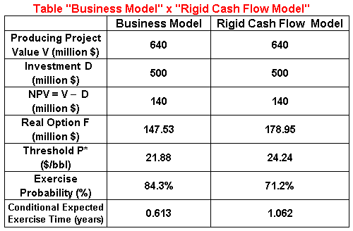
The table below presents results from a numerical example
of a real options with two years to expiration (for the default values in
the Timing spreadsheets for both models), with the same values for the
producing project value (V), investment (I) and Net Present Value (NPV).
This table shows that the Business Model is more conservative in terms of
real option value. However, it is less conservative in terms of the option
to invest exercise because it recommends earlier exercise than the Rigid
Cash Flow Model.
Although applicable also to the Rigid Cash Flow Model, the
concept of economic quality of reserve was first thought for the Business
Model because it is the multiplicative factor on the oil prices in order
to get the value of one barrel of developed reserve.
So, for more details on the Business Model and its applications, see the
webpage on economic quality of reserve.
The equation for the producing project value V(P) in the "Rigid Cash Flow Model" is given by the equation:
V = q' B P - C
Where q' is the economic quality of this reserve (because it is the partial derivative of V in relation to P, per barrel). The reserve volume is denoted by B, and C is a present value of part of the operational costs. The remaining part of the operational cost (like royalties) is embedded in q', as we will see later.
The net present value (NPV) for this model is:
NPV = q' B P - C - D
There are similar models in the real options literature. For example:
Let us discuss a typical discounted cash flow analysis for the NPV. In
order to keep things simple, assume that the discount rate
r is the same for all project flows (revenues
and costs) after the option exercise (a similar reasoning is
possible using different discount rates).
By grouping the cash flows using our equation NPV = V -
D, where V is the presented value of the revenues net of operational costs
and taxes, and D is the present value of the investment net of
fiscal benefits associated to the investment (net of depreciation
and others fiscal benefits). The equation for V deserves more details.
In this way, we can write the following equation for V:

Where Q(t) is the production at the year t; P(t) is the oil price; ROY is the royalties rate (generally between 10 - 15%); VOC is the variable operational cost (chemical products, transport costs, etc.); FOC is the fixed operational cost (maintenance cost in the wells and processing plant, wage costs with the operators, etc.); tc is the corporate income tax rate; r is the discount rate; and tabd is a (fixed) abandonment year.
Note in the equation above that the first term inside [.] is the revenue net of royalties, the second one is the variable operational cost, and the third one is the fixed operational cost. We can separate the above equation into three terms as follows:

For simplicity, in addition we assume that the (stochastic) long-run price
P in the above equation is constant (after the option
exercise) or P represents a weighted average price (first years are much
more important due to both Q(t) profile and discounting effect). Of course
is possible to use the curve E[P(t)] to calculate the first term, but it
costs computational time and loses analytical facilities (e.g., it is not
possible to use the analytical approximation for American calls options).
In this way we can isolate P and other terms which are not function of
the time in the equation above, writing:

Comparing the above equation with the "Rigid Cash Flow Model" equation for V(P) = q' B P - C, the first term (in red) corresponds to q' B P, and the summation of the remaining terms (in blue and in violet) corresponds to C (the terms without P). The term in blue corresponds to the variable operational costs, whereas the term in violet are the fixed operational costs.
This means that, in the Rigid Cash Flow Model, the quality factor q' is a function of the royalties, the income tax rate, and the discount rate. In this case the Economic Quality of a Reserve q' for the Rigid Cash Flow Model is given by:

Because the summation with Q(t) alone is exactly the reserve volume B. It is easy to prove that q' < 1 for positive values of the parameters of the above equation.
By looking the blue term in the last equation for V, it is obvious that the operational cost factor C is also related with the reserve volume B. What about the last term (the violet one)? Although it is not visible in the equation, it is also related with the reserve volume B. Why? Remember that the fixed operational cost is related with the capital in place, that is, it is (an increasing) function of the number of wells and the size of the production system (platform size, etc.). So, as in the case of the development investment D, the operational cost factor C is also an increasing function of the reserve size B and we can write C(B) in real options applications like the ones related with the value of information (models with technical uncertainty).
For this case, we can write the equation for the operational factor C as:

In practice, the easiest way to find the factors q' and C is by performing the sensitivity analysis of the NPV with P in a discounted cash flow spreadsheet. With resulting linear equation for the NPV x P, the intercept is - C - D, whereas the angular coefficient is q' B. Return to the introduction to linear models and see the linear chart NPV x P, in order to remember this point.
Let us relate the value of real option to invest in the project F with
the stochastic variable oil price P for the "Rigid Cash Flow
Model". We want the partial differential equation (PDE) for the value
of real option F(P, t). This option expires at t = T and the
exercise earn the payoff:
NPV = q' B P - C -
D
In the contingent claims method (see Dixit & Pindyck, for example) we need to construct a riskless portfolio F relating the option F with the stochastic variable P. Assume an imaginary portfolio buying one option F and selling short n units of P (or n barrels of oil). The value of this portfolio is:
F = F - n P
The value of n will be conveniently chosen in order to make riskless this portfolio (delta hedge). In this way, the riskless return of this portfolio in a small interval dt is given by:
r F dt = r ( F - n P ) dt
But the portfolio return is also the algebraic sum of the
return from its individual components.
The variable F return is related only to capital gain (it doesn't pay
dividends). This capital gain in a small interval dt is denoted by
dF.
The return of the variable P in a small interval dt has two components,
the capital gain dP and the dividend d
P dt, where in d is the convenience yield
of this commodity (or rate of return of shortfall). So, the portfolio
return is also:
r F dt = dF - n (dP + d P dt)
Equaling the two equations:
r ( F - n P ) dt = dF - n (dP + d P dt) . . . . . . . (*)
The value of dF is given by the Itô's Lemma expansion for F(P, t):
![]()
Where the subscripts denote partial derivatives. If P follows a geometric Brownian motion (GBM), elementary stochastic calculus tells us that (dP)2 = s2 P2 dt, we have:
![]()
Substituting dF into the returns equation (*), we obtain:
![]()
Rearranging, we get:
![]()
We want that the portfolio return, given by the equation above, be riskless. This means that we need to eliminate the stochastic term with dP (which is function of dz) to get a riskless return. This is easily performed by choosing the value of n = FP in the above equation. So, we obtain:
![]()
Rearranging we finally get the PDE for the real option F in function of the stochastic variable P:
![]()
There are interesting coincidences with the above PDE.
First, in financial options, if P is the price of a stock, the above PDE
is the exactly the famous Black-Scholes-Merton equation (version with
continuous dividends)! Second, the reader can verify that the PDE for the
"Business Model" is exactly the same above!
Why? This PDE only relates the option value F with P. Note that until
this point, the payoff equation that distinguishes the "Rigid Cash
Flow Model" from the "Business Model" was not used yet.
As in many options models cases (but not all), the differences are in the
boundary conditions:
a) for P = 0, F(0, t) = 0
b) for t = T (expiration), F(P, T) = max (q' B P - C - D, 0)
c) Value matching: for P = P* (where P* = threshold for
optimal immediate investment),
F(P*, t) = q' B P* - C -
D
d) Smooth pasting: for P = P*, FP(P*, t) = q' B
However, if both the operational cost C and the development
investment D are constants (given the expected values for q' and B), we
can solve the "Rigid Cash Flow Model" using the software that
solves the "Business Model"!
How? Look the differences, the boundary conditions. If we call V' = q'
B P = V + C and also D' = D + C, we can use for example our
Excel spreadsheet Timing
to solve the "Rigid Cash Flow Model" (available to download
below).
Using V' and D', we can use even the concept of homogeneity of degree 1 described in Dixit & Pindyck (p.210) because V' is proportional to P. For the case of costs (both C and D) this property helps to solve many problems (like the one related to value of information with constant values for the cost C and investment D). This is because we can use a normalized threshold curve [V'/D'(t)]* = [(q' B P*(t))/(D + C)] to fasten the problem solution.
However, when including stochastic costs the situation
is very different. In order to hold the degree 1 homogeneity is
necessary to assume that D' (= C + D) evolves according a (correlated with
P) geometric Brownian motion. The concept of homogeneity will not apply to
D itself (imagining either C constant or following other stochastic
process). The intuition behind is simple. If we double P and D but not C,
the NPV will not be the double, and so the option for the cases when F =
NPV. However, if P, C and D are doubled, the NPV will be the double.
The harder to accept assumption that C + D follows a GBM (in order to
take advantage of the homogeneity) is the main disadvantage of the
"Rigid Cash Flow Model" compared with the "Business Model".
For the case when P, C and D follow different (correlated) stochastic processes, even GBMs, the real options PDE, F(P, C, D, t) can be complicated to solve by finite differences. In this case, recent techniques of Monte Carlo simulation for American options looks the best practical way to solve this problem.
The Excel spreadsheet below, shareware available to download, is the Timing Version Rigid Cash Flow Model, which calculates real options, threshold, probability of exercise, and expected first-hitting time conditional to exercise, using the "Rigid Cash Flow Model". It considers that the (long run expectation on) oil prices follows a geometric Brownian motion (GBM).
![]() Download the Excel spreadsheet Timing
Version Rigid Cash Flow Model (timing-rcf_model-vba-hqr.xls), with
703 KB
Download the Excel spreadsheet Timing
Version Rigid Cash Flow Model (timing-rcf_model-vba-hqr.xls), with
703 KB
![]() Or
download the compressed (.zip) version of this spreadsheet
Timing Version Rigid Cash Flow
Model (timing-rcf_model-vba-hqr.zip), with 637 KB
Or
download the compressed (.zip) version of this spreadsheet
Timing Version Rigid Cash Flow
Model (timing-rcf_model-vba-hqr.zip), with 637 KB
The only limitation of this spreadsheet compared with the registered version, is that some inputs are fixed in this non-registered version. The fixed inputs are: Initial oil price; investment cost; operational cost factor; risk-free interest rate; and dividend yield (or convenience yield). Registered users can freely change any input.
Again, the table below presents results from a numerical
example of a real options with two years to expiration (for the default
values in the Timing spreadsheets for both models), with the same values
for the producing project value (V), investment (I) and Net Present Value
(NPV).
This table shows that the Rigid Cash Flow Model is less conservative in
terms of real option value. However, it is more conservative in terms of
the option to invest exercise because it recommends later exercise than
the Rigid Cash Flow Model.

The chart below presents the typical sensitivity analysis NPV with the oil prices P, for the fiscal regime of production sharing. This fiscal regime is used in many countries (mainly in Africa). Remember that for the fiscal regime of concession, this chart is a straight line.
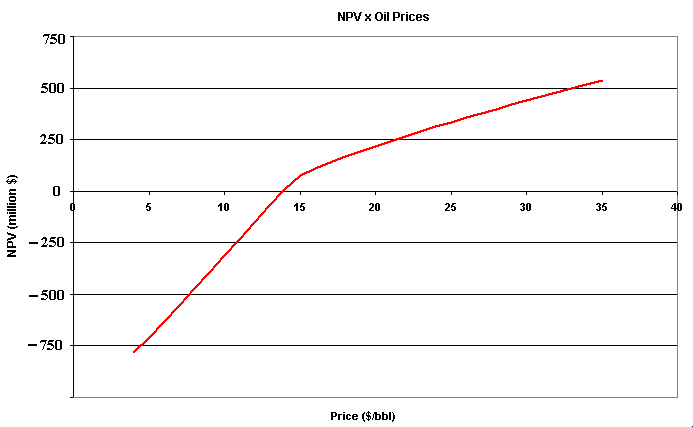
The production-sharing regime has two main phases, and the
figure above illustrates these two different phases. The first one is
named cost recovering, so that the revenues net of operational
cost from the first years are destined to the oil companies, in order to
recover the amount invested in the petroleum field (in general considering
an interest like Libor plus x%). In this phase, the Government Take
(GT) is inexistent or very small.
The second phase, named profit phase, the revenues net of
operational cost are destined to both Govern (larger part) and oil
companies. It seems like two different regimes, if the project (ex-post)
has no profit, the GT is zero or very small, whereas for ex-post
profitable projects the GT is significant.
Remember that for the regime of concessions, profit or non-profit project
is an oil company problem. Even with negative NPV, the oil companies pay
royalties, income tax (if the company is profitable, doesn't matter the
project), and other taxes. In the regime of production sharing, the
taxation changes at the point that the project enters in the profit phase,
causing the nonlinearity.
In the figure, if the oil price is under $ 15, the project has lower fiscal charge because it stays in the cost recovering phase, but for higher prices the fiscal charge is heavier because the project reaches the profit phase. This change of regimes is not at the NPV = 0 level because the discount rate used in the NPV estimate above is different of the discount rate used by the National Agency to reward the investment for cost recovery rule purposes.
This case is a bit more complex to simulate, but it is not so critical. It requires a complete specification of the NPV function variation with the oil prices (like the above chart) and with the others variables of interest (like reserve volume, productivity of the reserve, etc.).
For the model developed in the book of Dixit & Pindyck,
chapter 6 (p.188, eq.12), we have the value of the underlying asset V(P)
considering a nonlinear term due to the (costless) option to shut-down
the production if the price P drops below the unitary operational cost c.
The NPV equation is equal to V(P) less the investment I.
Although the textbook cash-flow function max(P -
c, 0) is too simple, the model permits to develop the intuition on the
effect of the shut-down option in both the NPV and the option to invest.
This intuition generally holds in more complex cases.
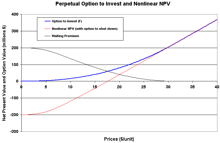
The chart below presents an example of the NPV equation with the option to shut-down.:
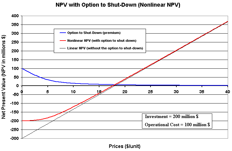
The case in the book refers to a project with infinite production life. This assumption permits an analytical solution for the NPV with the (costless) option to shut-down. For projects with finite life, including the option to shut-down will demand a numerical solution for the partial differential equation that determines the value of the underlying asset V(P, T), and so the NPV = V - I.
The Excel spreadsheet below, which the reader can download,
calculates the NPV with the option to shut-down and generates the above
chart.
In addition, it permits to calculate the value of a perpetual option to
invest in this project (the option to wait and see, see Dixit &
Pindyck p.190), generating also the chart for the perpetual timing option
presented below.
In this case the payoff from the exercise of the option to invest in the
project, is the NPV of the project including an option to
shut-down (this spreadsheet doesn't use macros or VBA and is not password
protected).
![]() Download the Excel spreadsheet dp-chapter6-nonlinear_npv.xls,
with 108 KB
Download the Excel spreadsheet dp-chapter6-nonlinear_npv.xls,
with 108 KB
This spreadsheet also illustrates the application of the Newton-Raphson method to solve nonlinear equations. In the above spreadsheet, this method gets automatically the value of the threshold P* and consequently the value of the real option F.
The chart of the perpetual option to invest with the price P is displayed below.
