Uncertainty in Demand Curve

Suppose that the demand of some product, rather than the output price, is the main source of uncertainty. The market of a generic product has demand curve P = f(q), where P is the price and q is the demanded quantity.
The output price is linked to the demand curve due the very known inverse demand curve.

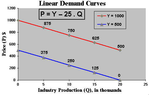
The following figures illustrate two very known demand curve, the linear demand curve and the exponential demand curve.
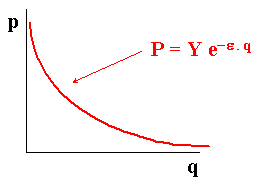
Consider an exponential demand curve with elasticity e:

Now consider two linear demand curves curve the same inclination but with different levels in function of the demand factor Y:

A problem with this approach is that, even if the linear demand is defined in a restrict production range so that the price is positive, with a negative stochastic variation of Y the positive price could become negative (a problem of economic consistency).
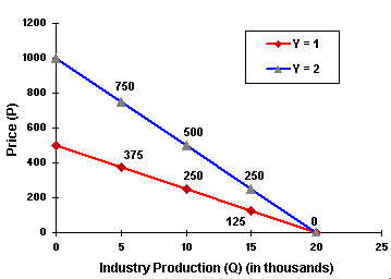
In order to prevent this, one alternative is to consider a multiplicative demand shock Y. For example by using the equation:

P = Y (500 - 25 Q)

With Y(t) following a geometric Brownian motion, so that if (500 - 25 Q) is positive for a range of Q, then the price will be positive because Y cannot be negative.
The starting value of Y, could be unity, that is, Y(t = 0) = 1. The figure below shows the linear demand curve with multiplicative stochastic shock passing from Y = 1 to Y = 2.

The linear demand curve has the advantage of the simplicity, but it permits zero or negative prices for large supply values (for Q equal or higher then 20 in the above example).

A good alternative is the iso-elastic inverse demand curve, which in the simplest format is given by: P = 1 / Q. However, iso-elastic demand has the following drawback: the total revenue = P.Q is constant, so that the industry (monopoly or oligopoly in tacit collusion) in presence of variable operational costs will find optimal reduce the production to near zero (with prices going to infinite) in order to reduce the operational cost without decreasing the revenue! This cause mathematical problems.
One solution is analyzed in the interesting paper of Agliari & Puu (2002), where they suggest the modified iso-elastic inverse demand curve: P = 1 / (Q + W), so that the hyperbola is translated to a new position intersecting the ordinate-axis - so that the maximum price is 1/W when production tends to zero.

Suppose that the factor Y is uncertain, fluctuating with time. So the demand curves can be in different places with a time. The following figure shows two exponential demand curves for differents values of Y.

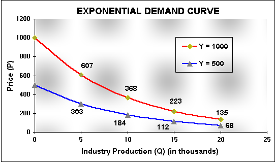
The current demand function is known (Y = Y₀) but the future demand function P = Y D(q) is uncertain.

Note that the exponential demand curve doesn't allow negative prices if Y doesn't assume negative values.
This suggest the use of lognormal distribution for Y.
Other interesting feature is the proportionality, if the Y drops x percent, the price P drops also x percent.

Usually the uncertainty on the demand factor Y is modeled with a lognormal diffusion process. Let Y to follow a geometric Brownian motion (GBM):

dY/Y = a dt + s dz

A good feature of multiplicative demand shocks, that is, P = Y . k, where k can be a deterministic demand function, is: if Y follow a GBM then the price P also follows a GBM and with the same parameters like drift and volatility! The vice-versa is also valid.
For the proof, see the webpage on "Business Model" in the topic named "Proof that V Follows the Same Geometric Brownian Motion of P".

For real options applications where the demand is uncertain (instead the prices), the threshold for an optimal investment will be at the threshold demand level Y*.

For a demand uncertainty applications see some applications at the option games webpage.