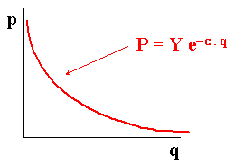
The model of duopoly under uncertainty is based in Dixit & Pindyck book (1994, chapter 9, last section), but with some practical adaptation:
This is an option-game application. See other related applications in the option-game webpage.
For a software related to this theory, go to the Duopoly under Uncertainty Spreadsheet webpage, from the real options software section.
OBS: This webpage is under revision, in order to consider many additional aspects and a more rigorous discussion on equilibrium strategies. The revision is coming soon!
The market of a generic product has (inverse) demand curve given by P = f(q), where P is the price and q is the demanded quantity. Consider an exponential demand curve with parameter e which is a kind of elasticity.

This type of inverse demand curve has the some advantages over other more popular inverse demand curves. For example, the linear inverse demand curve can lead to negative prices for high output production.
A good alternative is the iso-elastic inverse demand curve, which in the simplest format is given by: P = 1 / Q. However, iso-elastic demand has the following drawback: the total revenue = P.Q is constant, so that the industry (monopoly or oligopoly in tacit collusion) in presence of variable operational costs will find optimal reduce the production to near zero (with prices going to infinite) in order to reduce the operational cost without decreasing the revenue! This cause mathematical problems.
One solution is analyzed in the interesting paper of Agliari & Puu (2002), where they suggest the modified iso-elastic inverse demand curve: P = 1 / (Q + W), so that the hyperbola is translated to a new position intersecting the ordinate-axis - so that the maximum price is 1/W when production tends to zero.
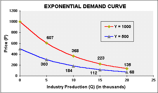
Suppose that the factor Y is uncertain, so the inverse exponential demand curves can be in different places along the time. The following figure shows two demand curves for different values of Y.
Modelling the factor Y uncertainty with a lognormal diffusion process, let Y follow a geometric Brownian motion (GBM):
The current demand function is known but the future demand function P = Y D(q) is uncertain. The uncertainty is modeled with a GBM for the oscillations in the demand factor Y. Its current value is known (Y = Y0).
Let us examine a leader-follower duopoly under uncertainty, extending the Smets' model presented in the Dixit & Pindyck book.
For example, suppose there is a duopoly in a telecommunications market.
Consider one small city with telecom investment opportunity. Both firms,
leader and follower, have a perpetual option to invest in that market with
stochastic demand.
Firms have rational expectations and maximize value under demand
uncertainty, expressed in the factor Y.
The current demand function is known but the future demand function P = Y
D(q) is uncertain and modeled with a GBM (see item 2 above).
Let we allow different unitary investment costs for firms, so the leader has a cost I1 per unity of product and the follower has a cost I2 per unity of product. So, I extend the model to permit cost differentiation between the players.
The valuation is performed backwards, first you should first calculate
the follower value, supposing that the leader already entered.
Given that follower behavior, the leader value is calculated. This means
that the leader value will be affected by the expected entry of the
follower (when the demand rise until the threshold Y2).
The follower has a perpetual option to entry in the market, producing q2, and waiting the demand increase until reach a threshold level Y2 where is optimal the immediate investment of the follower (threshold for the follower).
The demand curve is for the industry, so consider the sum of the both firms production, that is,
P = Y e- e q = Y e- e (q1 + q2)
Suppose that the price P is net of operational expenses, so that P can
be interpreted as a margin (profit).
To simplify, imagine that the present value of the operating project V is
the result of a perpetual flow from this profit P:
V = q2 . P/d, where
d is the dividend yield or the rate of cash
flow distribution given by:
d = r - a
With the presented premisses we can calculate the threshold Y2 and the follower value F2, for a perpetual option:

Where:

If Y > Y2 the follower value is:
F2 = q2 (Y e - e (q1 + q2))/d - q2 I2
If Y < Y2, the follower will wait until the demand factor
reach for the first time the threshold level Y2. The expected
time to occur that is called first hitting time T* of the
stochastic process of Y.
When this happen, the follower will get the same anterior value for F2,
but discounting with the rate r, since this
will happen in T*.
The expected value for the discount factor E[e- r T*] is given below:
E[e- r T*] = (Y/Y2) b1
See the Appendix A, Proof for the First Expectation for the demonstration and details.
So, the follower value is:

A typical call option value chart represents the follower value.
The leader will, for a certain time (until T*), remain acting alone in the market, without the follower. So, the demand curve is:
P = Y e- e q = Y e- e (q1)
After the time T* the leader profit will be shared with the follower
that, entering at this instant, will change the demand curve to:
P = Y e- e q = Y e-
e (q1 + q2)
The value of the expected cash flow, discounted by the rate r until the moment that the follower enters, added to the expected present value after the follower entry, gives the leader value F1:
If Y > Y2 : F1 = q1 Y e- e (q1 + q2))/ d - q1 I1
If Y < Y2, the leader knows that the follower will wait until the demand shock Y reach the threshold Y2. The value of the leader is given by the present value of the expected cash-flow producing alone in the market until T* plus the expected cash-flow after the follower entry at T*, less the investment cost to become a leader. This is given by the expression below:

Is necessary the first hitting time concept to calculate the
expectations (for the expectation of the integral, see the
Appendix B "Proof for the Second
Expectation" and for the other expectation, see
Appendix A).
By substituting the results from the appendixes (and remembering
d = r - a) we get:
Leader Threshold Y1
If the firms are equal (same cost) and if becoming leader doesn't mean a
larger market share (same q), we have the case analyzed in Dixit &
Pindyck chapter 9.
In this case the threshold value Y1 is given by the point that
both firms are indifferent to assume the leader or follower role. This
happen when F1(Y1) = F2(Y1)
provided that Y1 < Y2 (because at Y2
again the leader and follower values are equal). Of course, use the F2
equation for Y < Y2.
Equaling these two equations, F1(Y1) = F2(Y1),
we get a nonlinear equation for the threshold Y1. Use the
Newton-Raphson method to find the root Y1 or other methods
(like the "goal seek" facility from Excel).
The following picture shows the leader and follower values and the entry
thresholds:
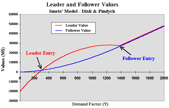
The above chart is built with homogeneous firms in the sense of same
unitary cost I and producing the same quantity (the firms have the same
market share of 50%).
This is very similar to the chart presented in Dixit & Pindyck (1994,
p.311).
In case of first move advantage in the sense that the leader
obtains a larger market share, the threshold Y1 is
given by the point that each firm is indifferent between the leader and
follower roles, but this time at Y1 the value of leader
producing q1 > q2 is equal to the value of the
follower that (probably) will produce in the future a lower quantity q2.
That is, F1(Y1, q1) = F2(Y1,
q2).
The chart below presents this case of different quantities or different market shares. In this case the leader gets a higher market share and produces q1 = 15,000 units, whereas the follower produces q2 = 10,000 units.
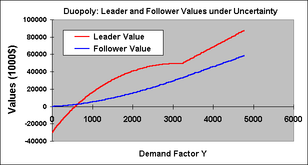
The leader and follower points are as before, but when the follower
enters the leader value is higher because his/her higher market share.
Note also that, with both in the market, the inclination of value line of
leader is higher than the follower. This means that when the demand rises,
the leader value grows more than the follower value. But when the demand
value decreases, the leader valuer drops faster than the follower.
Note also that in order to produce a larger quantity the leader
investment is larger because the larger capacity demands more investment
(remember that the leader investment = I1 q1).
Hence the threshold Y1 can be larger than the previous case.
Here is not allowed incremental investment in capacity. If we allow an
option to expand production, the leader could invest in a
small capacity at lower threshold Y1 in the first stage, with
the option to expand the production at a later moment (but the follower
could invest before the leader exercise of the option to expand). This is
a more complex case, which is left for a future extension.
Let us examine the case of different costs between the players but with the same market share. Suppose I1 = 1500, lower than I2 = 2000, so that there is a competitive advantage for the first firm.
In this case the leader will be the firm with the lower cost, because
the point of indifference between leader and follower roles for the firm
with lower cost Y1(1) is lower than the point of
indifference for the firm with higher cost Y1(2).
In this case, the firm with lower cost doesn't need to invest at Y1(1)
because the threat of the other firm entering the market is believable
only at the level Y1(2).
The entry threshold Y* for the firm with lower cost will be some point in
the interval: Y1(1) < Y* < Y1(2).
The chart below present this case of different costs and same market shares.
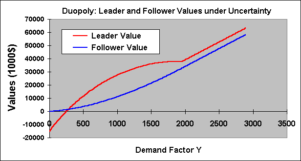
In the above chart the firms produce the same quantity q1 = q2 = 10,000 units.
Let us allow both different market shares and different costs. The chart below shows this case.
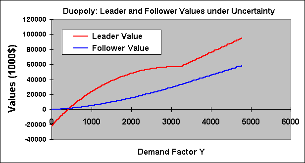
The final question is to set the optimal quantities q1 and q2
for the leader and follower.
For the Stackelberg equilibrium, the leader commit a production level q1 and the follower reacts according firm 2 reaction curve function q*2(q1).
There is a discussion if the Stackelberg equilibrium is the most likely outcome or if it is the Cournot-Nash equilibrium.
Stackelberg outcome is possible if we assume a immutable capacity commitment by the leader. However, if the game continues it is not Nash equilibrium because there exists an incentive for the leader to reduce its production in order to maximize profit. After this, the follower will react in the same way, until reaching the Cournot-Nash equilibrium (see the Appendix of the asymmetric duopoly webpage for a chart and additional issues).
Fudenberg & Tirole textbook (Game Theory, pp.74-76) points out that there is a problem of "time consistency" with the Stackelberg equilibrium, because the leader quantity in Stackelberg is not a best response for the follower production. In short, also in timing games with one firm entering before, the Cournot outcome is the most likely equilibrium.
So, let us assume that the most likely equilibrium is the Cournot-Nash outcome. The problem beconmes:
The follower maximize the profit given q1; and
The leader maximize profit given q2 = f(q1).
The follower profit is:
p2 = (q2 (Y e- e(q1 + q2))/ d) - I2 q2
By taking the partial derivative of the follower profit in relation to q2, and equaling to zero in order to get the optimal production q2, gives:
(e- e(q1 + q2) Y (1 - e q2)/d) - I2 = 0
The value of q2 is given for the above non-linear equation.
The solution can be found by an iterative process.
Note that the value of q2 is a function of the stochastic
factor Y.
Now is necessary to calculate the leader optimal quantity q1. This is done by looking the reaction curve q2 = f(q1).
p1 = (q1 Y e- e(q1 + q2))/ d) - I1 q1
Where q2 is given for the non-linear equation presented before, that is function of q1.
The solution is to find the maximum profit p1
by choosing q1.
One solution method is: in the calculus of optimal, for each q1
the value of q2 is calculated by the non-linear equation. With
these values is calculated a profit value p1.
By calculating several profits for each q1, is easy to choose
the higher one.
In this way are calculated the leader and follower values under
Cournot-Nash equilibrium for a given level of demand Y.
Things become more complicated if we invest in excess capacity in order to get the option to adjust the production output q1 to the oscillations in the demand level Y. This interesting complication is left for a future update.....
In this appendix I prove the expectation E[e-
r T*] = (Y/Y2) b1
by following the appendix in the chapter 9 of Dixit & Pindyck
textbook, but including some intermediate steps not showed in that book.
To make more general the notation, let the threshold Y2 =
Y*.
Suppose an expected discount factor in continuous time, with a generic (exogenous) discount rate r:
f(Y) = E[e- r t]
Denoting the first hitting time as T* (first time that Y is equal or larger than Y*), here representing when the option to invest will be optimally exercised, the expected discounted payoff from T* to current date is exactly the current value of the option to invest. Assuming that the current Y < Y* and by choosing an interval dt sufficiently small that hitting the threshold Y* in the next short time interval dt is an unlike event, the problem restarts from a new level (Y + dY). Therefore we have the dynamic programming-like recursion expression:
f (Y) = e- r dt E [ f (Y + dY) | Y] = e- r dt { f(Y) + E [ df(Y) ] }
By noting that:
(a) Y follows a geometric Brownian motion with drift a
and volatility s; and
(b) Using the Itô's Lemma for expanding df (Y), and using the
subscripts to denote derivatives we have:
df = fY (a Y dt + s Y dz) + 0.5 fYY (s2 Y2 dt) = fY a Y dt + fY s Y dz + 0.5 fYY s2 Y2 dt
Note that we are supposing the infinite time horizon (perpetual option)
case so that the variable time is not included in the Itô's Lemma.
By substituting df into the previous equation and by noting that E[dz] = 0,
and letting e- r dt = 1
- rdt for a very small dt, we get:
f (Y) = (1 - rdt) { f + fY a Y dt + 0.5 fYY s2 Y2 dt }
With a few algebra (remember dt2 is zero) the reader can find out the following differential equation:
0.5 s2 Y2 fYY + a Y fY - r f = 0
Where the subscripts denote derivatives. The general solution is:
f (Y) = A1 Yb1 + A2 Yb2
Where b1 and b2 are respectively the positive and the negative roots of the standard quadratic characteristic equation from the differential equation (see an instructive discussion of the characteristic equation in chapter 5, section 2.A, of Dixit & Pindyck book).
Applying two boundary conditions: as Y approximates to the threshold Y*,
T* is probable to be small and the discount factor f(Y) close to 1, so
f(Y*) = 1. When Y is close to zero, T* is likely to be large and so the
discounted factor close to zero, therefore f(0) = 0 (note: alternatively,
I think is possible to see Y = 0 as an absorbing barrier, so when Y tends
to zero, T* tends to infinite or there is no finite time for Y to reach
the threshold from Y = 0).
With these results, we can see that A1 = (1/Y*)b1
and A2 = 0.
Therefore the solution for the expected discount factor is:
Where Y is the initial value of the stochastic variable (that is at t =
0).
The parameter b1 is given by the
positive root of the fundamental quadratic equation (see Dixit &
Pindyck):

We want to prove the following result of the expectation below (defined by the function g(Y)), being T* the first time that the stochastic process (GBM) of Y reaches the threshold level Y*.

In the expectation of the integral, the main difference - when comparing with the first expectation - is that in the interval between 0 and dt there exists a dividend like profit p given by the value of the integral in this time interval:

Calculating the integral, we get:

Assuming that currently Y < Y* and by choosing an interval dt sufficiently small that hitting the threshold Y* in the next short time interval dt is an unlike event, the problem restarts from a new level (Y + dY). Therefore we have the dynamic programming-like recursion expression - this time including the profit or dividend-like term p(Y):
g(Y) = p(Y) + e- r dt E [ g (Y + dY) | Y]
The term p(Y) is calculated above and the term e- r dt E [ g (Y + dY) | Y] is calculated using the Itô's Lemma in the same way as calculated in the first expectation (see Appendix A above). Hence,
g (Y) = Y dt + (1 - rdt) { g + gY a Y dt + 0.5 gYY s2 Y2 dt }
With a few algebra it is easy to get the ordinary differential equation (ODE) showed in the chapter 9 appendix from Dixit & Pindyck book:
0.5 s2 Y2 gYY + a Y gY - r g + Y = 0
Where the subscripts denote derivatives. This ODE has a homogeneous part (equal to ODE from Appendix A) and a nonhomogeneous part (the last term of the left side in the equation above). The solution of this ODE is the sum of the homogeneous general solution with the particular solution:
g(Y) = B1 Yb1 + B2 Yb2 + Y / (r - a)
As before, b1 and b2 are respectively the positive and the negative roots of the standard quadratic characteristic equation
The value of the constants are calculated by using the boundary
conditions for Y = 0 and for Y = Y*. Look the definition of g(Y) for the
following reasoning.
For g(0) = 0 is necessary that B2 = 0;
For g(Y*) = 0 (because T* = 0) we get B1 = -
(Y*)1 - b1 / (r
- a).
Substituting the constants into the ODE solution, we complete the proof:
