Here is presented another application of the real options spreadsheets webpage from the real options software webpage.
This is an option-game application.
The model of duopoly under uncertainty is based in Dixit & Pindyck
book (1994, chapter 9, last section), but with some practical adaptation:
specifying the demand curve; allowing non-unitary production; allowing
leader and follower producing different quantities; and allowing cost
differentiation for the players.
For more details of the duopoly model,
go to the Duopoly
under Uncertainty Webpage which is a part of the
Option-Game Webpage.
OBS: This software is under upgrading in order to incorporate production optimization (optimal output for each firm), others demand curves, and additional equilibria analysis.
Older registered users will gain the new version for free. New registered users of Option Games Suite, will have the option to complement the software pack with 50% discount off the individual fee.
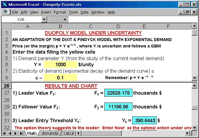
The figure bellow shows the main screen of the spreadsheet that solves this model. As in the Timing spreadsheets, there are an upper and a lower panel. In the upper one, the user put the data entry, seeing the results (values for the players for this figure) in the lower panel.

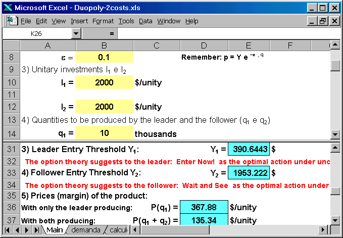
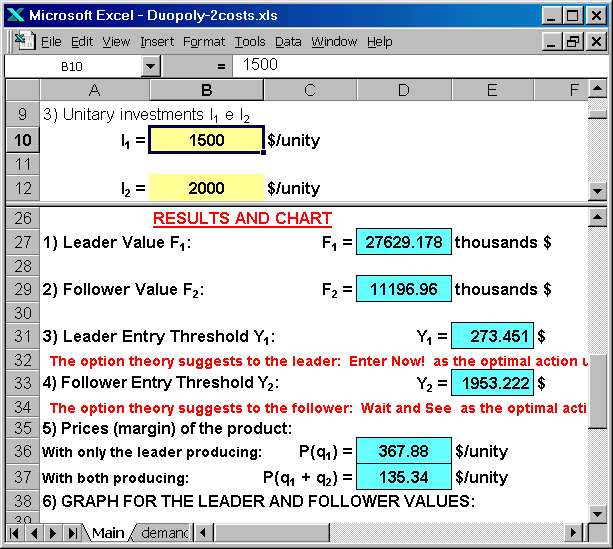
The following figure shows some details of the spreadsheet, like the investment costs for the players (upper panel) and the thresholds Y*, indicating according the current optimal action for the leader and the follower (lower panel). Also is calculated the prices for the case of leader producing alone and the case of both leader and follower producing.
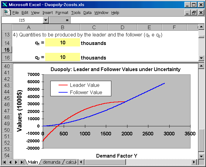
The next figure presents the quantity to be produced for the players (upper panel) and the chart with the players values. For Y > 1953, both players have the same value (in the Excel, although the blue and the red lines are superposing, only the blue line is showed).
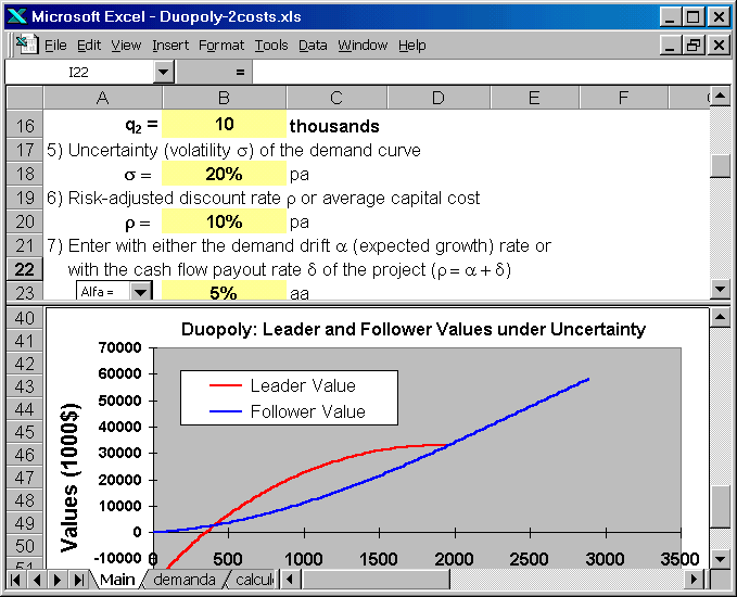
The next screen shows others parameters that the model needs, such as the volatility of the demand curve parameter Y, the risk-adjusted discount rate (interest rate for the risk-neutral case), the drift parameter (alternatively is possible to enter the dividend yield, but in practice the drift parameter is more used for the case of the demand uncertainty).
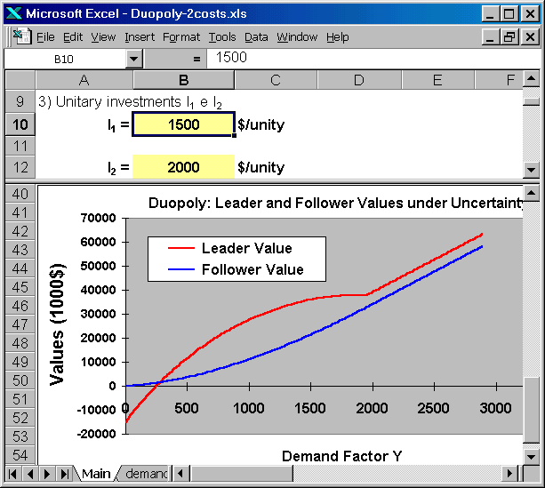
The figure bellow illustrates the case of investment cost differentiation (remained all the other parameters constant). In the lower panel is presented the effect on the players values. Even when both players are in the market, producing the same quantities, the leader value is higher due its lower cost.
The next figure illustrates the same case of investment cost differentiation but showing the numerical values for the players and also their thresholds in the lower panel (instead the chart presented in the last picture).
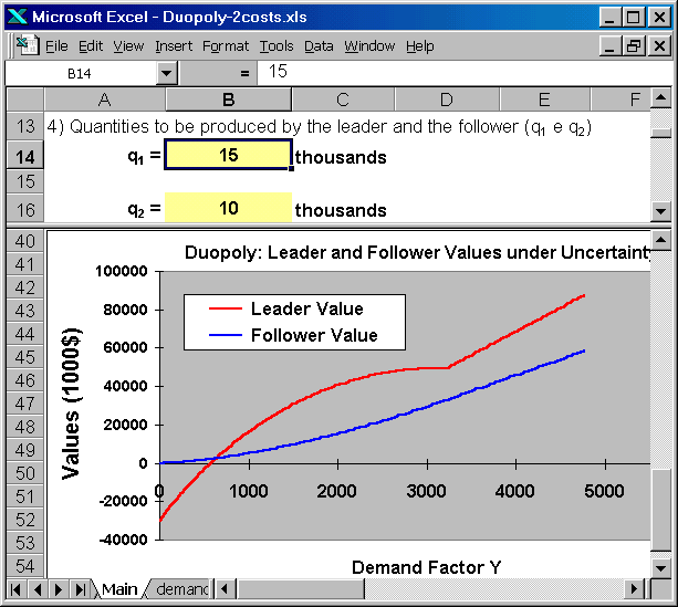
The screen below presents the case of different production quantities (or different market share) for the leader and the follower. For while, the costs are the same for both players. As in the case of cost differentiation, the leader value is higher but here the leader line has a higher inclination, getting a profit-leverage for the high-demand scenario.
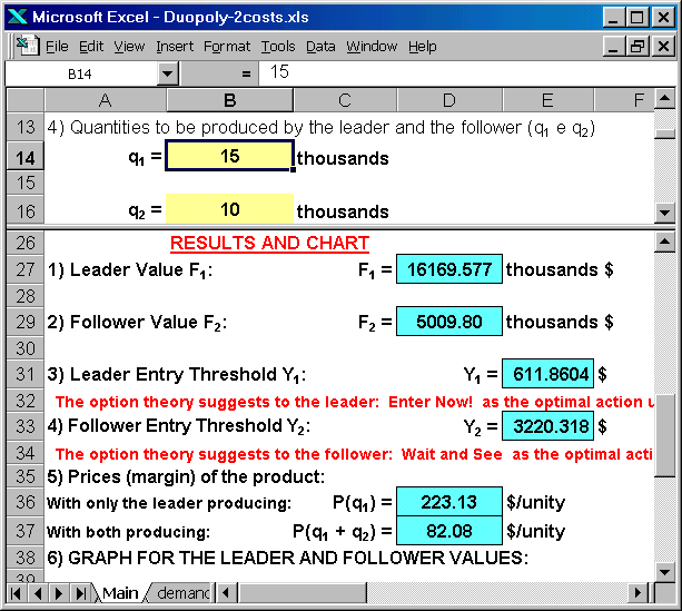
The next figure presents the same case of different market share (with same costs), but presenting the numerical results in the lower panel. Note that the entry threshold for the leader is higher than the first base case (comparing with the initial case, 612 versus 391), although the leverage is higher for high-demand case. You can think that the leader needs more scale to get that unitary investment cost, so the entry threshold is higher.
The following two screens present the combined case, the leader have both higher production (higher market share) and lower unitary investment cost. In the picture immediately below, is presented the chart, which looks like the different market share case but the numerical values are different.
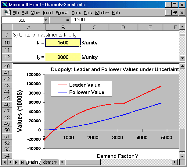
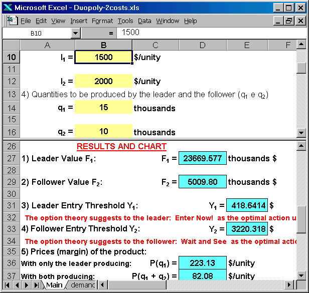
The picture below shows (lower panel) the values for the combined cost and market share differentiation. Note that the leader entry threshold is lower than the case of only market share differentiation (419 versus 612): the higher market share means also scale effect for the investment cost.
![]()