![]() 2) Model Assumptions, Monopoly, Cournot Duopoly and the Follower Value
2) Model Assumptions, Monopoly, Cournot Duopoly and the Follower Value
![]() 3) Leader Value and Threshold, and Simultaneous Exercise Value
3) Leader Value and Threshold, and Simultaneous Exercise Value
. . . . . . . . . . . . Numerical Example
![]() 4) Mixed Strategies Equilibria
4) Mixed Strategies Equilibria
![]() 6) Excel Spreadsheet: Contents and Download
6) Excel Spreadsheet: Contents and Download
![]() Appendix: Duopoly Equilibrium Possibilities and Reaction Curves
Appendix: Duopoly Equilibrium Possibilities and Reaction Curves
![]()
The Asymmetrical Duopoly under Uncertainty Model is a more realistic hypothesis in most industries. In the symmetrical duopoly model of Huisman & Kort, firms were homogeneous, whereas in this webpage the firms are different, there is an asymmetric duopoly. Here firms are non-homogenous because one firm has lower operational cost than the other for the same investment.
This means that one firm has competitive advantage over the rival.
In this webpage is described and extended the important and known model of Joaquin & Buttler ("Competitive Investment Decisions: A Synthesis", in Brennan & Trigeorgis, Eds., Project Flexibility, Agency, and Competition - New Developments in the Theory and Applications of Real Options, Oxford University Press, 2000, pp.324-339).
Following Joaquin & Buttler, we assume a linear inverse demand function, with quantities determined by a Cournot competition - firms choose quantities and the price clears the market according the inverse demand curve. Both firms are based in the same country and both are considering the investment in the same foreign country. The demand function is deterministic and fixed with the time. However, the exchange rate is uncertain and evolves as a stochastic process modeled as a Geometric Brownian Motion (GBM).
Although I get the same results, I consider the original paper development a little bit confusing, so that I follow a more traditional real options approach to get the paper results and some additional results.
This webpage try to answer some important questions mainly with charts and the Excel spreadsheet, describing and complementing the Joaquin & Buttler paper. The main questions are: What are the value of the firms as function of the exchange rate? What is the optimal policy for each firm for different exchange rate values? What are the Perfect Cournot Nash-Equilibria? Are there reasonable mixed strategy equilibria in this asymmetric duopoly?
The two main extensions of Joaquin & Buttler model are:
There are some other minor extensions, e.g., the value of the option to become leader.
Further extensions are planned for the future. For example, allowing other inverse demand curves; different investment values for the firms due to the different required maximum production capacity in this model; stochastic demand in addition to stochastic exchange rate, etc..
This webpage is divided into 6 topics. First, this introduction. Second, the model description, the assumptions, the monopoly case, the Cournot competition in duopoly, the follower value and threshold. Third, the leader value and threshold, the value of simultaneous exercise, and the original paper example with some charts to illustrate the asymmetric duopoly discussion. Fourth, the discussion on mixed strategies equilibria and the probability of mistake - simultaneous exercise when the optimal is only one investment with the leader and follower roles for the firms. Fifth, the analysis of equilibrium scenarios, indicating also the less probable but possible Perfect-Nash equilibrium. Sixth, this webpage concludes with the Excel spreadsheet, which is a component from the software pack "Options-Game Suite".
Warning: this page uses the Html 4.0 code for Greek letters. Use a modern browser for better understanding (Internet Explorer 5.5+ or Netscape 6+). If you are looking "σ" as the Greek letter "sigma" (not as "?", "s" or other thing), OK, your browser understand this Html version.
For the readers with older browsers, the alternative is to download the pdf version of this page (click here to download duopoly3.pdf), but the charts quality are not so good as this webpage.
Consider two firms, one named low-cost firm ( l ) and other named high-cost firm ( h ). Both firms are based in the same country and both are considering the investment in the same foreign country market. Firms can commit the same investment cost I to enter in the market, but their different variable operational costs makes the duopoly asymmetrical, with competitive advantage for the low-cost firm, due the lower operational cost compared with the high-cost firm.
Here, contrary the more general case of Huisman & Kort, the firms are not yet active in the foreign market, so that this is a "new market model" (see the webpage on Huisman & Kort model for this point).
The foreign country market inverse demand curve for the product offered, is linear and deterministic. The linear inverse demand equation is:
Where P(QT) is the price of the product in foreign currency, which is function of the total output in this market QT - the sum of both firms production. In order to make economic sense, the value of the constant "a" is sufficiently high so that only positive prices are considered.
In case of investment option exercise, exists a variable operational cost ci for firm i where i can be "l" or "h", for low-cost and high-cost firms respectively. The competitive advantage of low-cost firm is expressed by cl < ch .
The total operational cost Ci(Qi) for firm i is function its production Qi:
The function profit πi(Qi) for the firm i in foreign currency is:
The profit in domestic currency is given by multiplying the profit πi by the exchange rate X(t).
The exchange rate X(t) is stochastic and follows a geometric Brownian motion, given by:
The model assumes that firms are risk-averse but the risk-neutral contingent claims is possible by using for example a risk-neutral drift α' = r - δ and discounting with the risk-free rate r, with the dividend yield δ > 0 being interpreted as a foreign currency yield (see Joaquin & Buttler, p.329). The value of δ can also be estimated as the difference between the risk-adjusted discount rate for this business and the real drift of the exchange rate process.
Firms choose quantity and the price clears the market according the inverse demand curve. This is the named Cournot or quantity competition. See the nice paper by Kreps & Scheinkman (1983) on the comparison of Bertrand x Cournot competition, where the authors wrote that "Under mild assumptions about demand the unique equilibrium outcome is the Cournot outcome". In their paper with two-stage game, firms choose capacity (Cournot) in the first stage, and then follow a Bertrand competition in prices. The resulting outcome is the standard Cournot outcome! See also Varian, Microeconomic Analysis, 3rd ed., pp.301-302, for a discussion.
Why not the Stackelberg equilibrium? It is possible if we assume an immutable capacity commitment by the leader. However, if the game continues it is not Nash equilibrium because exists an incentive for the leader to reduce its production in order to maximize profit. After this, the follower will react in the same way, until reaching the Cournot-Nash equilibrium (see the Appendix).
Fudenberg & Tirole (Game Theory, pp.74-76) point out that there is a problem of "time consistency" with the Stackelberg equilibrium, because the leader quantity in Stackelberg is not a best response for the follower production. In short, also in timing games with one firm entering before, the Cournot outcome is the most likely equilibrium.
The optimal quantity will depend of the number of active firms in the market. First, let us see the monopoly case (only one firm, no threat of preemption) for comparison reasons and because in the duopoly the leader experiments a monopoly phase before the follower entry. After the monopoly result, is presented the asymmetric duopoly case and the equilibrium strategies.
The monopolistic firm i will choose the quantity that maximizes its profit function. It is a very simple maximization problem and the optimal quantity for the firm i in monopoly is:
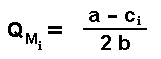
If the resultant value is positive. In case of negative value, the firm production is zero.
The profit flow for the monopolistic firm i is:
If the resultant value is positive. In case of negative value, the firm will not produce and the profit flow is zero.
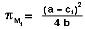
The optimal quantity in duopoly for one firm will depend of the both operational costs, the firm cost itself and the rival cost. The low-cost firm will produce more in Cournot equilibria than the high cost firm.
As before, this is a simple optimization problem, although here is a joint maximization problem. By taking the derivative of the profit in relation to quantity and equaling it to zero (first order condition) for each firm, we have the two best-response functions and the Cournot-Nash equilibrium is the crossing point - the simultaneous best-response point.
The optimal production quantity for the firms l and h are:
If the resultant values are positive. In case of any negative value, the firm production is zero.
The profit flows for the low-cost and high-cost firms are:
If the resultant values are positive. In case of any negative value, the firm will not produce and its profit flow is zero.
As standard in timing games, the solution is performed backwards. This means that first we need to estimate the value of the follower (given that the leader entered before), and then the leader value given that the leader knows the optimal follower entering can happen in the future. Here is considered that any firm can become the leader (the roles are not exogenously assigned), although is more probable that the low-cost firm will become leader and the high-cost firm will become the follower - however, we will see that the opposite is also Nash equilibrium, and in some cases the probability of simultaneous investment is strictly positive.
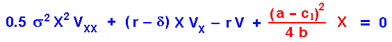
The follower value can be derived from the traditional real option approach. It is a perpetual American option to invest as follower, obtaining the follower cash flow in perpetuity.
There is at least other way to find the follower value, using the expected discount factor at the first time that the stochastic process hits the follower threshold. I will use the traditional differential approach, but the format of the follower equation will be easily identified by the adepts of the other approach.
The follower value in domestic currency is given by the known differential equation (subscripts denote partial derivatives):
The solution can be obtained with the usual method - the boundary conditions at the follower threshold, namely the value-matching and the smooth-pasting.
With these conditions, the follower value for the high-cost firm is given by (for the less probable low-cost firm as follower, just permute the subscripts l by h and vice-versa):
Where β1 is the positive (and > 1) root of the quadratic equation 0.5 σ2 β2 + (r - δ - 0.5 σ2) β - r = 0. See Dixit & Pindyck for a nice discussion on these quadratic equations for the homogeneous part of the differential equation. OBS: here and in most cases on option-game section, the term with other root, the root β2 < 0, is zero due to the usual limiting considerations when the underlying stochastic variable goes to zero. The negative root is relevant only in problems with abandon option, temporary stopping, lower reflecting barrier and similar situations.
The format of the follower value equation when the exchange rate is below the threshold has natural interpretation. The first term, between [.], is the NPV from the option exercise at X*Fh. The second term, multiplying the first one, is the expected value of the stochastic discounted factor, from a random time of the follower exercise T*Fh. Recall from other option-games webpages that the expected value of the stochastic discount factor for the first time T* that the stochastic process X(t) reaches a threshold XF is:
The follower threshold for the high-cost firm X*Fh is given by (for the less probable low-cost firm as follower, just permute the subscripts l by h and vice-versa):
The follower strategy is to invest at the time T* = TF = inf (t | X(t) ≥ X*F).
The figure below presents the follower curves for both high-cost and low-cost firms, illustrating the smooth-pasting condition at the follower thresholds. Of course the investment threshold for the high-cost firm is higher than the low-cost firm threshold. In the main equilibrium, of course the high-cost firm will be the follower.
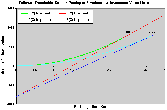
The parameters used in this figure come from the paper example. These parameters are showed in the ending of the next topic, see the sub-topic "Numerical Example".
There are at least two ways to calculate the leader value, by using the concept of first hitting time as in Dixit & Pindyck or by writting the differential equation of the leader during the monopolistic phase. I will use the latter approach, but for the equivalence between the two approaches, see the page on the symmetric duopoly of Huisman & Kort.
Consider the differential equation of the value of the leader during the monopolistic phase, for the low-cost firm as leader Vl (for the less probable high-cost firm as leader, just permute the subscripts l by h). This value needs match the value of simultaneous investment (= follower value) at the boundary point X = XFh. The differential equation of the leader value during the monopolistic phase in domestic currency is:
The solution is the general solution for the homogeneous part (blue part of the differential equation) plus the particular solution for the non-homogeneous term - the cash-flow. The latter is here just the profit flow from the monopoly phase in domestic currency. The solution is (again, for the less probable high-cost firm as leader, just permute the subscripts l by h and vice-versa):
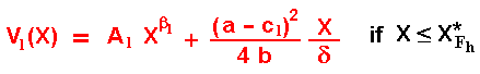
The constant Al is function of the firm, if low-cost or high-cost. It is the parameter that remains to be calculated, requiring only one boundary condition for that. This constant Al is negative, reflecting in the (expected) leader value the losses due to the probable follower investment exercise. This is mathematically showed below.
The relevant boundary condition is the value-matching at the point that the follower entry (at XFh). The smooth-pasting condition is not applicable here because this point is not an optimal control from the leader, it is derived of one optimization problem but from the other player. This boundary condition is:
The low-cost firm leader value during the monopolistic phase is equal to the simultaneous investment value at XFh. Equaling the two last equations, and after a few algebra, the value of the constant for the low-cost firm is easily obtained (again, for the constant of the high-cost firm, just permute the subscripts l and h):
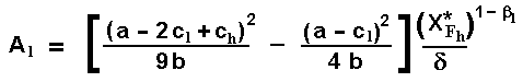
Although this constant is exactly the same of the paper (eq.16.6e), the format is much more heuristic due to the difference on the profit flows format - it permits quicker extension to other demand functions.
With this format, it is easy to see that this constant is negative: we know that the profit flow from the duopoly phase is lower than the profit flow from the monopolistic phase.
The negative value of the constant means that the leader value function is concave. This means that the effect of the follower entering is to decrease the leader value, as expected by the economic intuition in this duopoly.
The low-cost leader value in the monopoly phase Vl(X) is obtained by substituting this constant into the leader equation.
Let define the value of becoming a leader as L = V - I. In reality, both Dixit & Pindyck and Huisman & Kort, denote L the leader value (but not Grenadier, 2000) probably because it permits a direct comparison of L with F in the choice of the optimal strategy (and to check the incentives to deviate of strategy).
If X < XFh, the leader value defined as L = V - I, for the low-cost firm is given by:
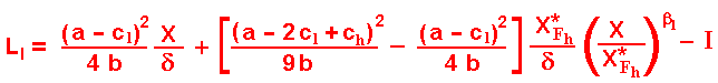
The format of this equation also permits an intuitive explanation. The first term of the right side is the monopoly profit in perpetuity of the leader firm. The middle term is the expected present value of the competitive losses, which will occur at the follower entry (decreasing the monopoly profit in perpetuity) . The last term is the investment required to become leader.
Again, for the less probable high-cost firm as leader, just permute the subscripts l by h and vice-versa.
For X ≥XFh, the leader value is equal its simultaneous investment value, because both firms are producing in the market.
Let us take the opportunity to define the simultaneous investment value for the low-cost firm as function of the stochastic demand shock X, denoted by Sl(X), as:
Again, for the high-cost firm, just permute the subscripts l by h and vice-versa.
The value of simultaneous investment is important because it is necessary to answer fundamental questions like: (a) what if I deviate from the follower waiting strategy by investing? and (b) I want to become a leader, but what if the rival has the same idea at the same time and both invest simultaneously?
In other words, it is necessary to check if a follower strategy is a Nash-equilibrium and the expected value (or expected losses) if by "mistake" both invest at the same time (this will be important for the calculus of mixed strategies equilibria).
Note that the simultaneous investment can be the optimal policy for both if the state of demand is so high that X ≥ XFh, but a mistake in case of X < XFh. The chart from a numerical example soon will show this issue in a clear way.
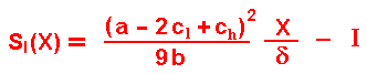
Without the preemption menace, the firm will invest optimally at the monopoly threshold XMl. However, due to the menace of preemption, firms cannot wait so far to invest. If one firm wait until X = XM, in some cases the other firm can invest at XM - ε, but the first firm could preempt the rival by investing before when X = XM - 2 ε, etc. This process stops when one firm has no more incentive to preempt the rival.
Firm l has incentive to become leader if Ll > Fl but it is not necessary to invest at this point because the low-cost firm knows that high-cost firm has incentive to become leader only if Lh > Fh . So, low-cost firm strategy to become leader is to invest when Lh = Fh.
The figure below show this issue - see the next sub-topic "Numerical Example" for the input data, the low-cost firm has incentives to enter when Ll > Fl, that is, when X > 0.88. However, without menace of preemption of the rival, low-cost firm will prefer to invest later (at XMl if possible). But, in this example there is menace of preemption from the rival (high-cost firm) at the level X = 1.03, so that the low-cost firm leader threshold is XLl = 1.03, which is also equal the high-cost firm leader threshold, XLh = XLl = 1.03:
In this case XLl is the value of the stochastic exchange rate where Lh(XLl) = Fh(XLl) and XLl < XFh.
In other cases, depending mainly on the difference between the operational costs cl and ch, the competitive advantage could be higher disappearing the menace of preemption before X = XMl. In this case the competitive advantage is so high that the low-cost firm ignores the competition by investing at the monopolistic threshold XMl - this is named open-loop strategy.
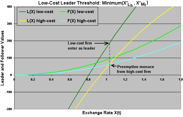
The last chart used the base-case parameters, with ch = 21 F$/unit (F$ = foreign currency). If we increase this cost - increasing the competitive disadvantage of the high-cost firm, is possible that the follower rôle for the high-cost firm be always better than the leader rôle. The base-case example but with ch = 23.5 F$/unit, is displayed in the chart below, showing the follower, leader and simultaneous investment curves.
In the above chart the follower curve (light blue) is always above the leader value. In this case it is always better for the high-cost firm to be the follower - never is optimal be the leader, waiting until the exchange rate reach the level X*Fh = 5.44 in this case.
For the rival low-cost firm, this means that there is no menace of preemption so that the low-cost firm can ignore the competition by investing at the monopolistic threshold XMl.
So, the leader threshold is the minimum between its monopolistic threshold and the other firm minimum level with incentive to become a leader. This is essentially the "Result 3" from the Joaquin & Buttler paper.
Let us illustrate the mathematical development with a numerical example and additional charts. The base case of the example is the same of the paper of Joaquin & Buttler.
The base-case parameters are (percentage in annual basis):
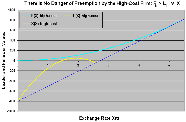
The only chart presented in the paper is showed below. It is a non-conventional chart in option-games literature because it doesn't tell about the leader preemption threshold and because the X-axis is not the exchange-rate: the X-axis represents the entry threshold Xe. The idea is to see the entry threshold that maximizes the firm values. The drawback is that it doesn't consider the preemption menace in the leader value functions.
The chart shows, for both firms, the monopolistic thresholds - the leader curves maxima, and the follower thresholds - the follower curves maxima. However, the leader curves are non-conventional also because these curves are conditional to the optimal entry of the other firm as follower.
The interesting thing in the chart above is that, because the (strategic) leader thresholds are also indicated in the chart, is possible to compare the entry option premium (the NPV when entering) for the case of the monopoly - about D$240 for the low-cost firm and D$140 for the high-cost one, with the option premium for the case of duopoly - entering at the (strategic) leader threshold, about D$175 for the low-cost firm and D$60 for the high-cost one.
So, the effect of the duopoly is to decrease the NPV at the optimal enter level, in relation to the monopolistic case.
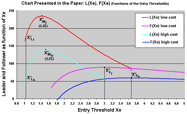
The chart below presents all the curves from the base-case example. Namely, the leader, the follower and the simultaneous exercise value curves for both the low-cost and high-cost firms (6 curves).
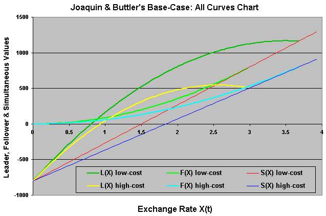
I presented before only some of these curves and with a zoom in the interest region in order to identify clearly the strategic details of this asymmetric game.
Next, we will discuss the necessity to consider mixed strategies for some cases and the equilibrium possibilities.
Now, imagine that the initial state of the exchange-rate is so favorable that both firms have incentive to become leader because exists an exchange-rate region where L > F for both firms. However, both firms will be worse in case of simultaneous exercise of the option to invest because the value of simultaneous investment is even lower than the follower value, namely S < F for both firms.
It is obvious that, without communication between the firms, there is a positive probability of "mistake" - simultaneous investment getting a value lower than the follower one. The figure below shows this region. Note that if the high-cost firm has incentives to become leader - that is the case showed in the figure below, the same happen with the low-cost firm. However, we know that the vice-versa is not necessarilly valid.
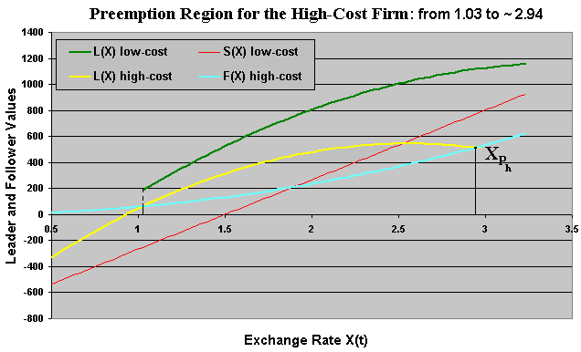
Let us denote the region above as Preemption Region for the High-Cost Firm. The existence of this region depends on the parameters, specially the difference between the costs, that is, the competitive advantage value. In the base case this region exists. This means that the low-cost firm in this region suffers the risk of obtaining the simultaneous value (red line in the above chart) instead the "logical" or "natural" leader value when investing (green curve in the chart). This risk must be considered when analyzing this game.
The high-cost firm threat is credible, because if the high-cost firm enters first, the best for the low-cost firm is to resign with the follower rôle, unless X ≥ XFh. We will see later that it is also a Perfect Nash equilibrium, although less probable.
Define XPh as the preemption upper bound from the "Preemption Region for the High-Cost Firm", see the figure above. In the chart above this upper bound is approximately equal to 2.94. This upper bound will be used soon in the mixed strategies theorem. The lower bound of the region - about 1.03 is the leader threshold (equal for both firms).
Remark: There is no logic to imagine that, without any communication, the other firm will let the rival to become leader in the above case. Both firms will wish the higher leader payoff, but both firms fear the possibility of becoming worse in case of simultaneous investment (a "mistake ").
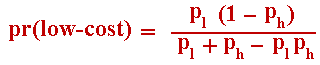
As in Huisman & Kort model, the desire to become leader (or the probability to invest) is proportional to the difference between the L and F values and decreases if the difference between F and S increases. This means that, for this preemption region with positive probability of simultaneous investment, the probability of option exercise for the low-cost firm is strictly higher than the probability of option exercise for the high-cost firm. Even lower, this probability is positive in this region. We need to calculate this risk!
In order to determine the mixed strategies probabilities, I use partially the Theorem 8.1 from the Huisman's textbook ( "Technology Investment: A Game Theoretic Real Options Approach", Kluwer Academic Pub., Boston, 2001, p.204). He analyzes the asymmetric duopoly case (chapter 8), but it is a little bit different from our case because the asymmetry in the book occurs with different investments, whereas here the investments are the same and the asymmetry is due to the different operational costs.
(a) Consider the scenario with parameters so that exists a non-empty Preemption Region for the High-Cost Firm.
Define the following probabilities of exercise pl(X) and ph(X) for the low-cost and high-cost firms respectively:
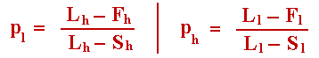
Readers of the webpage on symmetrical duopoly model of Huisman & Kort will recognize this format and know how to find out results like that using the concept of "atoms" and a maximization process. Note that these probabilities are functions of the opponent payoffs. These probabilities are the equations 8.18 and 8.19 from the Huisman's book. In a previous version of this webpage I wrongly claimed that these equations were inverted. The book equations were correct even not being intuitive at first look (probabilities of exercise are independent of our payoffs, they just depend on the opponent payoffs). The intuitive explanation is that we set a probability so that the opponent keeps indifferent between exercising or not her option. In this way, she cannot exploit my strategic exercise probability. Mathematically, these probabilities result from the first order conditions for both expected payoffs, Vl and Vh in relation to the probabilities pl and ph, respectively.
Now consider the following possible cases of initial value for the stochastic exchange rate X(t = 0):
(a.1) If the current exchange rate X(0) belongs to the "Preemption Region for the High-Cost Firm", then with probability:
low-cost firm invests immediately and high-cost firm invests when X reaches XFh.
With probability:
high-cost firm invests immediately and low-cost firm invests when X reach XFl.
And, with probability:
both high-cost firm and low-cost firm invest immediately, the named probability of mistake.
(a.2) If the current exchange rate X(0) is lower than XLh (that is, at the left of the "Preemption Region for the High-Cost Firm") and lower than XMl, then with probability one low-cost firm invests when X(t) reach XLl = minimum(XLh, XMl ) and high-cost firm invests when X reach XFh.
(a.3) If the current exchange rate X(0) is lower than XLh and higher than XMl , then with probability one low-cost firm invests immediately and high-cost firm invests when X(t) reach XFh.
(a.4) If the current exchange rate X(0) is higher than XPh (that is, at the right of the "Preemption Region for the High-Cost Firm") and lower than XFh, then with probability one low-cost firm invests immediately and high-cost firm invests when X reach XFh.
(a.5) If the current exchange rate X(0) is higher or equal than XFh - that is, a region where is optimal for both firms to invest, then with probability one both firms invest immediately.
(b) If the Preemption Region for the High-Cost Firm is an empty set (there is no X that L > S for high-cost firm), then:
Low-cost firm will invest with probability one at XMl as leader (alone) and high-cost firm will invest with probability one only at XFh, as follower.
Readers of the webpage on symmetrical duopoly model of Huisman & Kort will find out the way to prove the item (a.1) of this theorem using the steps presented there. For the other items, just observe that there are no incentives to deviate from the above strategies, with both firms maximizing their expected payoff.
Next, let us see the equilibrium analysis charts on the firms values in function of the exchange rate.
Collusion: Recall the discussion in the Huisman & Kort's model: because this is a "new market model" collusion is never an equilibrium here. Here, in addition, the firms' asymmetry makes tacit collusion unfeasible as equilibrium even if they were active in the market before. So preemption is always the equilibrium scenario here.
The chart below represents the value functions for the main Perfect-Nash equilibrium, with the low-cost firm with the role of leader and the high-cost with the role of follower for the relevant exchange rate region.
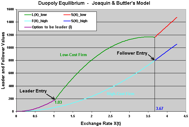
In the chart above appears a new value function: the option to become leader. This value function is easily calculated if we have the leader threshold XLl, by using the expected value of stochastic discount factor from the random time to X(t) reaches the leader threshold, times the leader value function for the low-cost firm showed before.
The chart below represents the value functions for the secondary or less probable Perfect-Nash equilibrium, with the high-cost firm with the role of leader and the low-cost with the role of follower for the relevant exchange rate region.
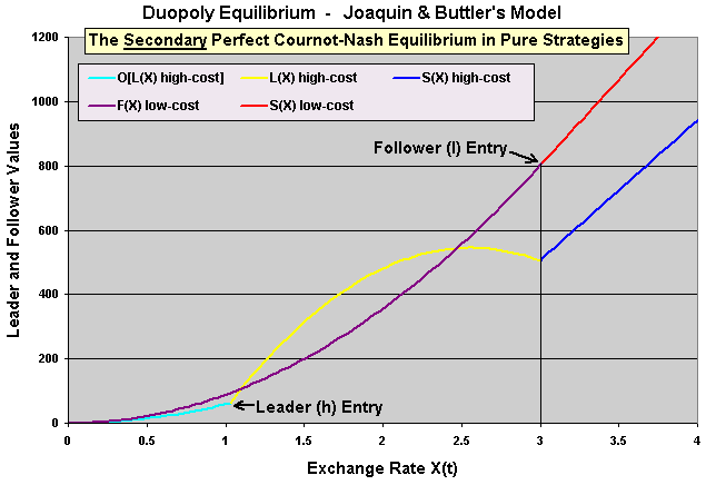
Let us explain better why high-cost firm entering as leader is a "less probable Perfect-Nash equilibrium" considering the results presented before. If X(t = 0) < XLl, the probability of either high-cost firm becoming a leader and simultaneous investment are zero. This means that almost surely the secondary equilibrium from the above figure will not take place (even not being impossible). However, if in the market beginning (t = 0) the exchange rate X(t=0) > XLl and X(t=0) < XFh, depending on the parameters the probability of secondary equilibrium occurrence is strictly positive but lower than the occurrence probability for the main equilibrium (so, the secondary equilibrium remains less probable).
Recall that, depending on the parameters, exists the possibility of a simultaneous investment situation when the optimal for both firms is only one firm active in the market. If this simultaneous exercise happens - a mistake with positive probability if the initial exchange rate is in the preemption region for the high-cost firm, the deviation is not possible because the investment is irreversible.
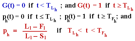
As in Huisman & Kort's, the equilibrium strategies are given by the pair of cumulative probability of exercise by (at least) one firm, given that the other firm has not invested, G(t) and the instantaneous exercise probability of the firm "i" pi(t).
Recall from Huisman & Kort's model that when the instantaneous probability pi(t) becomes positive, the cumulative probability goes to one because an instantaneous simultaneous game, which can be repeated without consuming time and with possibly infinite rounds, is played. In this repeated game each player i = l, h, has probability pi(t) to exercise the option in each round.
Denote the time for X reaching the thresholds XF and XL as TF = inf (t | X(t) ≥ XF) and TL = inf (t | X(t) ≥ XL), respectively. Additional subscripts "l" or "h" denote that the time in question refers to low-cost firm or high-cost firm, respectively. However, we see before that XLl = XLh.
For the low-cost firm, we have the following specification for the mixed strategies equilibria G(t), pl(t):
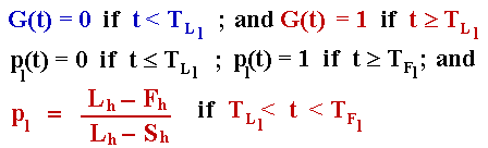
For the high-cost firm, we have the following specification for the mixed strategies equilibria G(t), ph(t):
The Excel spreadsheet below is the non-registered version of a component of the Option-Games Suite. See the page on real options software for the registration fee and the details on how to register.
The non-registered version is equal the registered version except that some inputs are fixed and the page with the calculation details is hidden and password protected. However, all the examples and variations discussed above can be reproduced with the non-registered version by changing some non-protected inputs.
The registered version gives the freedom to change any input and there is no protection in the registered file, with all sheets unhidden, including the sheet with the detailed calculations. The extensive use of names for cells eases the user to follow the calculations in all the spreadsheet, including the sheet with the calculations details.
The Excel spreadsheet has the following sheets:
The non-registered version can be freely downloaded below and used for educational purposes:
![]() Download Excel file named duopoly-ext_joaquin_buttler-non-reg.xls with 1,508 KB or
Download Excel file named duopoly-ext_joaquin_buttler-non-reg.xls with 1,508 KB or
![]() Download Compressed (.zip) Excel file named duopoly-ext_joaquin_buttler-non-reg.zip with 889 KB
Download Compressed (.zip) Excel file named duopoly-ext_joaquin_buttler-non-reg.zip with 889 KB
This spreadsheet is a component from the software pack Option-Games Suite. The registered version the sheet of calculus is non-protected and the registered reader can see the calculation details>
See how to register the real options software and the licence fees
In order to illustrates the different equilibriums, nothing better than a numerical example.
Imagine a linear inverse demand curve with p = 30 - (q1 + q2). Imagine that the variable cost is zero, in order to ease the calculus. Alternatively, we can think p as the margin instead price, so that the inverse demand curve addresses the firms profit margins.
The figure below shows the different possible equilibriums for this problem.
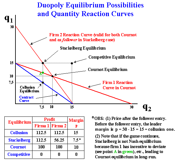
The figure above shows the reaction curves for the firms 1 and 2. Also is showed the contract curve with the collusion equilibrium. Note that without a binding contract, both firms have incentives to change the production level (it is not Nash equilibrium).
Note also that if the game continues, in the Stackelberg equilibrium case there also exists an incentive for the firm 1 to reduce the production (point A in green) in order to maximize profit (represented by the reaction curve). For duopoly case without collusive binding agreements, the most likely result is the Cournot-Nash equilibrium, which is time-consistent with no incentive to deviate.