![]() 2) Model
Assumptions, Monopoly Value, Duopoly and Follower
2) Model
Assumptions, Monopoly Value, Duopoly and Follower
![]() 3) Leader Value
and Threshold, and Simultaneous Exercise Value
3) Leader Value
and Threshold, and Simultaneous Exercise Value
. . . . . . . . . . . . Numerical
Example
![]() 4)
Mixed Strategies Equilibria
4)
Mixed Strategies Equilibria
![]() 5) Collusion
Value and Thresholds
5) Collusion
Value and Thresholds
![]() 6) Equilibria
Analysis: Collusion x Preemption
6) Equilibria
Analysis: Collusion x Preemption
![]() 7) Excel
Spreadsheet: Contents and Download
7) Excel
Spreadsheet: Contents and Download
![]()
The Symmetrical Duopoly under Uncertainty Model was the first known "option games" model (Smets, working paper in 1991 and doctoral dissertation in 1993), and was analyzed in chapter 9 of Dixit & Pindyck's textbook (1994). In addition to the historical relevance, this is model has a great theoretical importance - foundations of stochastic timing-games of preemption in continuous-time - and also practical significance for duopoly when there is no competitive advantage for one firm.
This section follows the in-depth analysis of this symmetrical duopoly performed by Huisman & Kort: "Effects of Strategic Interactions on the Option Value of Waiting", CentER Discussion Paper 9992, Tilburg University, September 1999, 41 pp. The paper is (or was) available to donwload from Tilburg University website.
This paper is a thorough (definitive?) analysis for this very basic
symmetrical option game. They extended the previous literature (Smets, Dixit
& Pindyck) in many ways, especially by allowing
mixed-strategies equilibrium and analyzing the possibility of
non-binding collusion equilibria. In addition, they presented many
propositions that establish the conditions for the occurrence of different
equilibria, in a rigorous approach.
With very few modifications, this paper
is also the chapter 7 from the very good textbook of Huisman on option-games in
continuous-time: "Technology Investment: A Game Theoretic Real Options
Approach", Kluwer Academic Pub., Boston, 2001.
I suggest the reading of the Huisman & Kort paper (or the chapter 7 of
Huisman's book), but the explanation here is self-contained - although
summarized in some topics - and it is complemented with many charts and an Excel
spreadsheet (which checks out all proposition, calculated values and tresholds,
presents charts, tell the optimal equilibrium, etc.). I provide also additional
explantions in some points of this model. The previous reading of chapter 9
(last section) of Dixit & Pindyck is also very useful.
The explanation
here presents only some minor modifications in notation of Huisman & Kort.
However, I include some issues not discussed in the paper or book, e.g., the
two ways to calculate the value of the leader.
This duopoly model is symmetrical in the sense that the players are
homogeneous firms (equal firms), so that this suggests symmetrical strategies.
I analyze the asymmetrical duopoly case in other webpage (model of
Joaquin & Buttler), when firms have different costs and so there is a
competitive advantage for the low-cost firm.
This webpage is divided into 7 topics. First, this introduction. Second, the model description, the assumptions, the monopoly case, and the follower value and threshold. Third, the leader value and threshold, including the two equivalent ways to calculate the leader value, the value of simultaneous exercise, and the original paper example with some charts to illustrate the duopoly discussion. Fourth, the discussion on mixed strategies equilibria and the probability of mistake - simultaneous exercise when the optimal is the leader/follower schema with only one investment exercise. Fifth, the value of collusion and the conditions for collusion without binding contracts. Sixth, the analysis of equilibrium scenarios, pointing out the more probable equilibrium scenario - collusion or preemption. Seventh, this webpage concludes with the Excel spreadsheet, which is a component from the software pack "Options-Game Suite".
Warning: this page uses the Html 4.0 code for Greek letters. Use a modern browser for
better understanding (Internet Explorer 5.5+ or Netscape 6+). If you are looking
"σ" as the Greek letter "sigma" (not as "?", "s" or other thing), OK, your
browser understand this Html version.
For the readers with older browsers,
the alternative is to download the pdf version of this page (click here to download
duopoly2.pdf), but the charts quality are not so good as this webpage.
The first difference of Huisman & Kort model - when compared with Smets /
Dixit & Pindyck - is that the two firms are already active in the
market producing one unit each, and they are considering the exercise of (a
definitive) one option to expand the production. This means that the "entry"
(read expansion) of a firm affects the current profit flow of the other firm -
reducing the profit flow because this model consider negative
externalities.
If firm 1 exercise the option by investing I and firm
2 doesn't invest, firm 1 is called the leader and firm 2 is called
the follower.
The firms face a (inverse) demand curve expressed by the profit flow P(t) for firm i given by:
P(t) = Y(t) D(Ni, Nj)
Where Y(t) is a (multiplicative) stochastic demand shock and D(Ni, Nj) is a deterministic demand parameter for firm i, which depends on the status of firms i and j. The possible values of D(Ni, Nj) are:
These factors D(Ni, Nj) are adjusted to the production
level. The operational cost is zero or it is also included in D, so that P is
interpreted as profit flow instead price.
For example, the profit flow of the
leader is Y.D(1, 0), and this profit flow is higher than Y.D(0, 0). That is, the
higher production level when investing and assuming the leader role, is already
included in the value D(1, 0). The change of status from D(0, 0) to D(1, 0)
demands the sunk investment of I.
In addition, due to the symmetry of the
problem, when one firm is profiting Y D(1, 0), the other firm is profiting Y
D(0, 1), etc.
For the called "new market model" - the original case of Smets and in Dixit & Pindyck, we have D(0, 0) = D(0, 1) = 0.
The stochastic demand shock Y(t) follows a geometric Brownian motion, given by:
dY = α Y dt + σ Y dz
The model assumes that firms are risk-neutral. However, it is easy and direct to extend the model to risk-averse firms in contingent claims approach by supposing that the stochastic process drift α is a risk-neutral drift. In practical terms, just let α = r - δ in the relevant equations presented below, with the dividend yield δ > 0. The value of δ can be estimated as the difference between the risk-adjusted discount rate and the real drift of the process.
The deterministic demand parameters have the additional constraint of negative externality given by the inequality:
D(1, 0) > D(1, 1) > D(0, 0) > D(0, 1)
Other assumption in Huisman & Kort's model is the first mover advantage, given by the inequality:
D(1, 0) - D(0, 0) > D(1, 1) - D(0, 1)
This inequality says that the gain when becoming a leader is higher than the gain when becoming a follower (for the same Y, and considering the same investment I).
Before any options exercise (when Y is below the leader threshold
YL), the value of each firm is the current cash-flow profit in
perpetuity, Y D(0, 0) / (r - α), plus the option to exercise the investment
option (as leader or as follower, with 50% each - as we will see later) net of
the competitive losses due to the negative externality from the rival
entry.
First, let us recall the monopoly case (only one firm, no menace of
preemption) for comparison reasons and because in the duopoly the leader
experiments a monopoly phase before the follower entry. After the monopoly
result will be presented the duopoly case and the equilibrium strategies.
In the monopoly case, we have the traditional real options problem, and the value of the firm V(Y) is the current profit plus the option to expand the production. The differential equation is given below, where subscripts means derivatives:
The blue part of the equation is the homogeneous part whereas the red term is
the non-homogeneous term (the cash-flow term) of the differential equation. For
the case of risk-averse firm, using contingent claims approach, just replace the
real drift α by the risk-neutral drift ( r - δ) in the
differential equation above.
The whole solution comprises the general
solution for the homogeneous part (option) plus the particular solution from the
non-homogeneous part (cash-flow), if the stochastic variable Y is below the
optimal exercise threshold for the monopolist YM. In case of Y equal
or higher the threshold YM, the value is the monopolist profit in
perpetuity net of the investment. See the equation below.

Where β1 is the positive (and > 1) root of the quadratic equation 0.5 σ2 β2 + (α - 0.5 σ2) β - r = 0. See Dixit & Pindyck for a nice discussion on these quadratic equations for the homogeneous part of the differential equation. Again, for the case of risk-averse firm, using contingent claims approach, just replace the real drift α by the risk-neutral drift (r - δ), so that the denominator (r - α) becomes equal to δ in the equations above.
The values of the constant A1 and the monopolist threshold YM are obtained with the value-matching and smooth-pasting conditions at the point where Y = YM (see for example Dixit & Pindyck for these typical boundary conditions). These values are:


The NPV from the option exercise at the threshold YM is ease to prove that is I / (β1 - 1), which is strictly positive.
As standard in timing games, the solution is performed backwards. This means that first we need to estimate the value of the follower (given that the leader entered before), and then the leader value given that the leader knows the optimal follower enter can happen in the future. Here is considered that any firm can become the leader (the roles are not exogenously assigned).
Note that the follower has a perpetual option to invest I and obtaining the
follower cash flow in perpetuity.
By following the usual steps, the follower
value is given by:

The values of the constant B1 and the follower threshold YF are as usual deternined by the boundary conditions value-matching and smooth-pasting. These values are:


Note that the constant B1 is positive reflecting the positive value of the option to invest as the follower. The function F(Y) is convex as consequence of the positive value of this constant.
The follower strategy is to invest at the time T* = TF = inf (t | Y(t) ≥ YF).
The leader value is a little bit more interesting. There are at least two ways to calculate this value. The first is to follow as in the paper and as in Dixit & Pindyck. The other way, not presented in the paper or in the Dixit & Pindyck, is perhaps simpler. Both are presented here (finding equal results).
The first approach divides the problem into two expectations. The monopolist
phase of the leader (when the follower has not entered yet), with high profits, and
the duopoly phase, when the follower entered and the leader profit flow drops
with the additional follower supply to the market. Let T* be the first time that
the path of the stochastic process of Y hits the threshold YF.
The figure below shows the leader value in this way:

We can write this equation as:

The calculus of these expectations with stochastic time T* is similar to the case presented in other page. These expectations value:
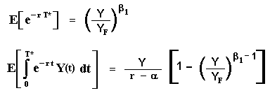
Click here for the proof of the first expectation and for the proof of the second expectation click here.
In this way, by substituting the results into the L(Y) expression we get the value of the leader as function of the leader optimal entry threshold, the parameters from the stochastic process of the demand, and the deterministic demand parameters in monopolist and duopolist phases, D(1, 0) and D(1, 1), respectively.
The alternative (easier!) way is to consider the differential equation of the value of the leader during the monopolist phase, denoted by V(Y) = L(Y) - I. This value V(Y) needs to match the value of simultaneous investment (follower value) at the boundary point Y = YF. So, it is ease to see that the differential equation of the leader value during the monopolist phase is:
The solution is the general solution for the homogeneous part (blue part of the differential equation) plus the particular solution for the non-homogeneous term (cash-flow). The solution is:

The constant B2 is the parameter that remains to be calculated,
requiring only one boundary condition for that. The biggest difference compared
with the constant B1 from the value of the follower, is that the
constant B2 is negative, reflecting in the (expected) leader value,
the losses due to the probable follower investment exercise. This is
mathematically showed below.
The relevant boundary condition is the
value-matching at the point that the follower entry (at YF).
The smooth-pasting condition is not applicable here because this point is
not an optimal control of the leader, it is derived of one optimization problem
but from the other player. This boundary condition is:
The leader value during the monopolist phase is equal to the simultaneous investment value at YF. Equaling the two last equations, we get:

The value of the constant is easily obtained:

Note that the constant value is negative because D(1, 1) < D(1, 0). This
means that the effect of the follower entering is to decrease the leader value,
as expected by the economic intuition in this duopoly. The negative value of the
constant means that the leader value function is concave.
The leader value in
the monopoly phase V(Y) is obtained by substituting this constant into
the leader equation.
Let define the value of becoming a leader as L = V - I.
In reality, both Dixit & Pindyck and Huisman & Kort, denote L the leader
value (but not Grenadier, 2000) probably because it is direct the comparison of
L with F in the choice of the optimal strategy (and to check the incentives to
deviate of strategy).
If Y < YF,
the leader value defined as L = V - I, is given by:

The reader easily can check this value is exactly the same obtained by the
first method (and we didn't calculate any expectation with random time).
If
Y ≥ YF, the value of becoming a leader is equal to the value
of becoming a follower, which is equal the value of simultaneous investment.
That is,

Let us take the opportunity to define the simultaneous investment value as function of the stochastic demand shock Y, denoted by S(Y), as:

In the paper, Huisman & Kort use the same notation of Fudenberg & Tirole for simultaneous investment value as M(Y). I prefer the notation S(Y) even because M can confuse with monopoly.
The value of simultaneous investment is important because it is necessary to
answer fundamental questions like: (a) what if I deviate from the follower
waiting strategy by investing? and (b) I want to become a leader, but what if
the rival has the same idea at the same time and both invest simultaneously?
In other words, it is necessary to check if a follower strategy is a
Nash-equilibrium and the expected value (or expected losses) if by "mistake"
both invest at the same time (this will be important for the calculus of mixed
strategy equilibriums).
Note that the simultaneous investment can be the optimal policy for both if the state of demand is so high that Y ≥ YF, but a mistake in case of Y < YF. The chart from a numerical example soon will show this issue in a clear way.
Without the preemption menace, the firm will invest optimally at the
monopolistic threshold YM. However, due to the menace of preemption,
firms cannot wait so long to invest. If one firm wait until Y = YM,
the other firm can invest at YM - ε, but the first firm could preempt
the rival by investing before when Y = YM - 2 ε, etc. This process
stops when one firm has no more incentive to preempt the rival
Firm 1 has
incentive to become leader if L1 > F1 and, most
important for firm 1 decision, firm 1 knows that firm 2 also has incentive to
become leader if L2 > F2 . So, firm 1 strategy to
become leader is to invest when L2 = F2. However, due the
symmetry of the problem, L1 = L2 and F1 =
F2 for all Y, so that the leader threshold is defined as
the Y in the interval 0 < Y < YF so that the values
of the leader and the follower are equal, i.e.,:
There is a proposition in Huisman & Kort showing that this Y (the leader
threshold) is unique. Due to the symmetry, this threshold is valid for
both firms.
The threshold notation YL is different of Huisman
& Kort. They prefer use YP for the threshold that I call
YL. The subscript "P" comes from "preemption". I prefer the simpler
notation of calling YL the threshold that the leader will enter in
equilibrium.
Let us illustrate the mathematical development with a numerical example and
charts. The base case of the example is the same of the paper of Huisman &
Kort.
The base-case parameters were
(percentage in annual basis):
Note that the non-stochastic demand factors obey both the negative
externalities and first-move advantage assumptions of the model.
In case of
risk-averse firm assumption we can think 5% as the risk-neutral drift in a
contingent claims approach.
The chart below presents the leader value, follower value, and the
simultaneous exercise value, as functions of the demand stochastic shock Y.
The chart also shows the leader threshold YL = 0.558 and
the follower threshold YF = 1.762.
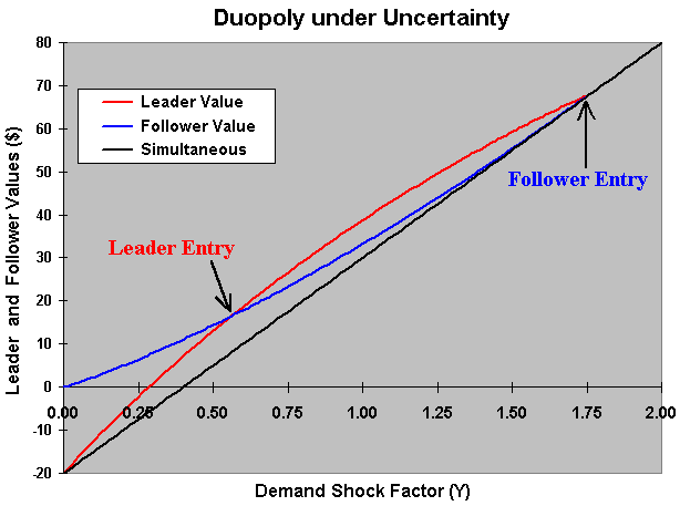
Now, imagine that the initial state of the demand is between YL and YF . Both firms have incentive to become leader because L > F (see the previous chart to clarify this point). There is no logic to imagine that, without any communication, the other firm will let the rival to become leader so that the probability of simultaneous investment is zero. Both firms will wish the higher leader payoff, but both firms fear the possibility of becoming worse in case of simultaneous investment (a "mistake"). The payoff from simultaneous exercise is lower even than the follower payoff.
Assuming non-communication between the players, the only rational way to
treat this problem in the game theory context is by allowing mixed strategies.
When communication is allowed - as suggested in Joaquin & Buttler (2000) -
there exists the alternative of a bargain-game (sharing the surplus L -
F) with agreement for only one firm to become leader in order to avoid the
"mistake" of simultaneous investment.
However, in many situations this kind
of agreement is illegal or contrary to accepted convention.
With mixed strategies, firms will rationally calculate the optimal probability to exercise the investment option aiming the leader payoff, but considering the positive probability of simultaneous investment. Firms will play a simultaneous game (possibly with infinite rounds) where the firm i can choose invest with probability pi and not invest with probability 1 - pi , players i = 1 or 2.
The analysis of mixed strategies in continuous-time preemption games, must be performed carefully and using special tools. The passage from discrete-time to continuous-time presents problems when using traditional limit considerations. Fudenberg & Tirole (1985) reported that the usual methods present "loss of information" in this passage, with the continuous case not representing the limit of the discrete case. In addition, with traditional tools many strategies converge with probability 1 to be played at the instant t = 0, a non-consistent result.
In order to determine the symmetrical mixed strategies, Huisman & Kort
used the same tool applied in Fudenberg & Tirole (1985): they specify
"probabilities" named of "atoms" p(τ) that, if positive,
indicate cumulative probability of exercise Gi(τ) equal to 1.
So, τ is defined as the first time that some player will exercise the option
to invest given that nobody exercised the option before.
This resource is
taken from optimal control literature (see for example Birge &
Louveaux, �Introduction to Stochastic Programming�, Springer Verlag, 1997,
p.289).
The fundamental idea is that this control doesn't take
time. Using this analogy, the control here is the result of a
simultaneous game that can be repeated. This is like an instantaneous
automatic optimizer. In this way, a simultaneous game with two players even
if repeated infinite times, is played instantaneously (no time consuming). This
approach determines the probabilities from the mixed strategies and is possible
to prove that this is the true limit of the equivalent game in discrete-time.
The simultaneous game, which can be repeated infinite times, at the instant that one (or both) player will exercise the option (that is, at τ), is showed in strategic form below, together with the probabilities of option exercise.
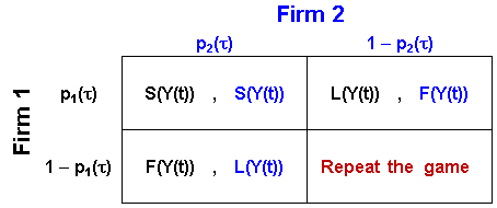
The firm 1 payoff, V1 (still not optimized) is given by:
The last term means that in case of repetition we get the payoff V1 due to the definition of τ: when this game is played (at τ, with infinite rounds) is certain that some player (or both) will exercise the option.
If you don't understand the equation above, an equivalent but perhaps more intuitive way is given by the equation below:
The term between the first [.] is the expected payoff of one round in case of definition (investment of one or two players). The second [.], in red, multiplies that expected payoff and consider the case of definition in the first round (multiplying by one), in the second round [multiplying by (1 - p1) (1 - p2) ], and etc., until infinite. The red term is just the infinite sum of a geometric progression with ratio lower than one (convergent), so that it is easily calculated. The reader is invited to check out the algebra in order to conclude that the two methods are equivalent.
Hence, the equation for the (non-optimized) payoff from the simultaneous game for the firm i, Vi, i = 1 or 2, is:

Next, players need to set the optimal probability to exercise the option,
that is, the probability that maximizes the expected payoff
Vi.
The first order condition for this optimization problem for
the firm 1 is ∂V1 / ∂p1 = 0, given the rival is
playing exercise the option with probability p2. It is ease to check
that the second order condition indicates a maximization problem (second
derivative is negative).
Note also that, due to the symmetry of the problem,
the optimal probabilities must be equal. That is, p1 = p2 = p*. This permits a
further simplification. Using the first order condition and the symmetry
insight, after some algebra we get the following simple equation for the optimal
probability of investing in mixed strategies:

The chart below presents a zoom in the previous chart (example from the last
section) in the region where there exists incentives for both firms to become
leader (L > F).
The figure gives a geometric interpretation for the
optimal probability of exercise p* in mixed strategies.
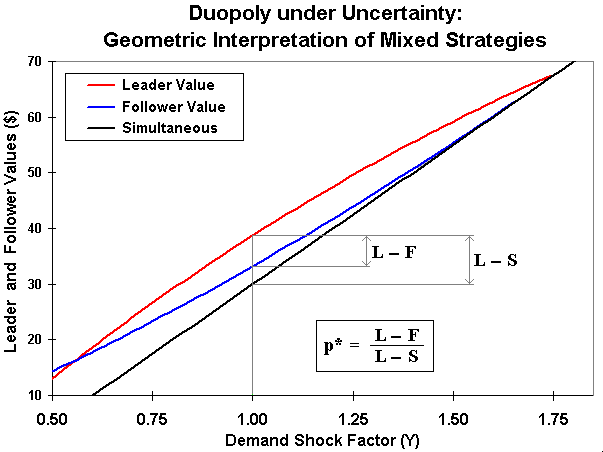
In the figure above, it is easy to see that when L = F and L > S, we have p* = 0. When L tends to both F and S, we have p* = 1. In the mixed strategy equilibrium, the probability p* can be interpreted as equal the ratio of the possible benefit from preemption (L - F) to the range of total possible variation (L - S) (note that L - S = [(L - F) + (F - S)]).
Now, let us calculate the probability of only one of the firms to exercise the option and the probability of simultaneous exercise in this game. For that, look again the figure with the strategic-form of the simultaneous game and, using a similar reasoning from the payoff, we can write that the probability pr(one = i) that only the firm i investing in one round from the simultaneous-game at τ is given by:
So, the probability pr(one = i) is:

Of course, the probability pr(one = j) of only the firm j investing in this
simultaneous-game at τ is exactly the same due to the symmetry.
Now, the
probability of simultaneous exercise (or probability of "mistake", if Y
< YF), denoted by pr(two), using a
similar reasoning is given by:

Note that the three probabilities sum one, that is, p(one = i) + pr(one = j) + pr(two) = 1. This is because there is no possibility of non-exercise in this simultaneous-game due to the definition of τ.
We can use the previous optimal value that we found for the probability p(τ)
= (L - F) / (L - S), and easily estimate the probabilities of each firm
investing and the probability of simultaneous exercise.
For example, at
YL we know that L = F and L > S. So, p(τ) = 0. In this case
pr(two) = 0 and pr(one = i) = pr(one = j) = 1/2.
Note that the probability of simultaneous investment is consistent in the limits when Y tends to YF or to YL :
Therefore, when the market births with Y < YL there are
50% chances each to became leader and zero probability of "mistake" when Y reach
YL. This conclusion from Dixit & Pindyck with trivial mixed
strategies outcome is correct only in this case, not in general as they claimed.
After reaching YL we have already defined the leader and the follower
and mixed strategy is not necessary anymore. However, only in this case the
mixed strategies developed above are not relevant.
For the case with market
birthing with YF > Y(t = 0) > YL, mixed
strategy analysis is essential and there exists a strictly positive
probability of mistake as we saw above. Huisman & Kort made this critic and
filled the gap by examining the general case with market starting with any
feasible value for the demand shock Y.
Denoting the time for Y reaching the thresholds YF and YL as TF = inf (t | Y(t) ≥ YF) and TL = inf (t | Y(t) ≥ YL), respectively, we have the following specification for the symmetric mixed strategies equilibria Gi(t), pi(t):

The symmetric strategies means that the above description of the equilibria is valid for both firms (i.e., i = 1 or 2).
Another interesting extension of Huisman & Kort is to consider the possibility of collusion equilibria without a binding contract between the firms (without communication). They analyze if there are situations that a tacit wait and see policy is equilibrium. Firms could calculate if is the best strategy or not the wait and see until one level Y = θ, when both invest simultaneously - or one firm invest and the other one invest immediately after that.
Collusion will only be Nash equilibrium if there is no unilateral
incentive to deviate. Deviation means to earn the leader payoff with the
other firm choosing optimally to invest much later as the follower.
We need
to calculate the collusion value of one firm waiting to invest simultaneously at
the level θ, denoted by C(Y, θ). In this case each firm will pass from
the demand status D(0, 0) directly to D(1, 1).
Collusion will be
Perfect-Nash equilibrium only if C(Y, θ) ≥ L(Y) at least for all Y in the
interval (0, YF).
With the usual real options steps (It�'s lemma, differential equation, boundary conditions, etc.), it is easy to reach the following value for one firm in collusion:

The Pareto optimal choice of the argument theta, will maximize the collusion value of each firm at θ = YC. In mathematical terms,
That is, the optimal collusion threshold YC (smooth-pasting condition at YC ) is:

This Pareto optimal is the most probable equilibrium outcome (if collusion is equilibrium) because if one firm invest before, there is a credible menace from the other firm to invest immediately after, obtaining a value lower than C(Y, YC ).
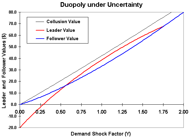
The chart below presents the leader value, the follower value, and the
collusion value as functions of the stochastic demand shock Y.
The
used parameters were the same of the previous charts. Note that the collusion
value is always higher than the leader one, so that the collusion equilibrium is
feasible (firms in collusion have no incentive to cheating). For the
base-case parameters, the collusion value curve smooth-pasting on the
simultaneous value line at YC = 5.287, a very high value so
that it is out of the chart.
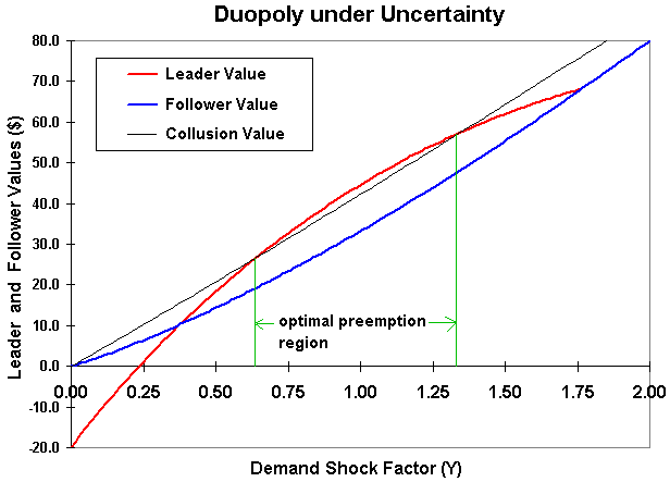
If the first-mover advantage is sufficiently large, the collusion can
be destroyed by the preemption.
The figure below illustrates this point. Now
the value of D(1, 0) = 5, which is higher than in previous case,
so that now there is a region where preemption is optimal due to the higher
value for the leader role when comparing with the collusion value. So, here the
firms in collusion have incentive to cheating and collusion is not
Perfect-Nash equilibrium.
The symmetric preemption equilibria from the last section remain being
equilibria (why?). In addition, depending of the parameters we can also have
infinite collusion equilibria.
For example, we can choose a θ =
YS < YC so that there is no incentive to deviate - it
is satisfied the condition C(Y, YS ) ≥ L(Y) for all Y in the interval
(0, YS). By defining TS = inf (t | Y(t) ≥
YS) and TC = inf (t | Y(t) ≥ YC ),
we have in this case infinite collusion equilibria by choosing the simultaneous
investment at the instant T* in the interval [TS, TC
].
As pointed out before, the Pareto equilibrium (at θ = YC
) is the more probable outcome from this infinite set of collusion
equibria.
As before, the equilibrium strategies are denoted by the pair of cumulative probability of exercise Gi(t) and the instantaneous exercise probability pi(t), which in this collusion case are:
An important result for the "new market model", that is, D(0, 0) = D(0, 1)
= 0, as in Dixit & Pindyck, the collusion value and the threshold are
both equal to the follower value and threshold. This means that collusion is
never equilibrium in the new market model. The curves of values of collusion
and follower coincide, so that preemption is always the equilibrium scenario
in the new market model.
While in the new market model the
investment timing of the leader does not change the follower profit flow, in a
more general model there exists a strategic interaction so that YF
< YC in the more general case - invest ealier to recapture market
share lost to the leader, and YC = YF for the new
market model.
The Huisman & Kort claims that being the threshold
YC equal the threshold Y3 from Dixit & Pindyck (Figure
9.2, p.311), this threshold must be equal to the follower threshold,
Y3 = YC = YF, not higher than YF as
showed in the book figure. This issue, Y3 = YC >
YF, can occur only in the more general model of Huisman & Kort. I
agree with Huisman & Kort.
The general definition if collusion is or not equilibrium depends on the
parameters of the problem and it is helped by two Huisman & Kort
propositions using functions f(β1) and g(β1).
Define
these functions as:


The authors proved that there are three possible equilibrium scenarios:
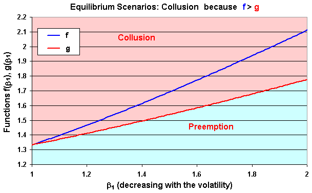
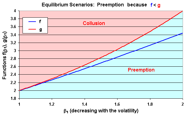
The next three charts below plot these functions f(β1) and g(β1), which define the collusion and preemption regions. See the propositions 3 and 4 from the Huisman & Kort's paper for details (or propositions 7.4 and 7.5 from the Huisman's book).
The first chart below is for the base-case used in most of the previous charts with D(1, 0) = 4. In this case, the blue line (function f) is above the function g for all the range of β1, indicating that collusion equilibrium is the most feasible equilibrium.
The chart below - the second case - is for D(1, 0) = 5. In this case, the blue line (function f) is below the function g for all the range of β1, indicating preemption equilibrium.
The chart below - the third case - is for D(1, 0) = 4.6. In this case, the blue line (function f) is above the function g for low values of β1 - indicating collusion equilibrium, and is below the function g for high values of β1 - indicating preemption equilibrium.
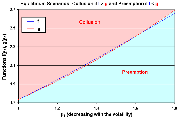
Remember that β1 is decreasing with the uncertainty (volatility σ), so that collusion equilibrium is more likely under uncertainty (β1 near 1) than in the deterministic setting from the seminal paper of Fudenberg & Tirole (1985). The figures above show this issue.
The Excel spreadsheet below is the non-registered version of a
component of the Option-Games Suite. See the page on real options software for
the registration fee and the details on how to register.
The non-registered
version is equal the registered version except that some inputs are fixed and
the page with the calculation details is hidden and password protected. However,
all the examples and variations discussed above can be reproduced with the
non-registered version by changing some non-protected inputs.
The registered version gives the freedom to change any input and there is no protection in the registered file, with all sheets unhidden, including the sheet with the detailed calculations. The extensive use of names for cells eases the user to follow the calculations in all the spreadsheet, including the sheet with the calculations details.
The Excel spreadsheet has the following sheets:
The non-registered version can be freely downloaded below and used for educational purposes:
![]() Download Excel file
named duopoly_hui-kort_non-reg.xls
with 791 KB
Download Excel file
named duopoly_hui-kort_non-reg.xls
with 791 KB
This spreadsheet is part of the software pack Option-Games Suite.
The registered version the sheet of calculus is non-protected and
the registered reader can see the calculation
details.
See how to register the real
options software and the licence fees