![]() 3) Oligopoly Simulation and the Spreadsheet Downloading
3) Oligopoly Simulation and the Spreadsheet Downloading
![]()
This section is based on S.R. Grenadier's working paper "Option Exercise Games: An Application to the Equilibrium Investment Strategies of Firms", Stanford University, November 2000. An almost equal version was published at Review of Financial Studies, vol.15, Summer 2002, pp. 691-721.
This paper has at least two very important contributions to the option-games literature:
Both insights simplify the problems solution because "the
exercise game can be solved as a single agent's optimization problem"
and the usual real options tools in continuous-time. In order to solve the
option-game problem it is not necessary more complex techniques to search
fixed-points from the players best-response correspondences.
It is not by chance that most contributions in option-games come
from real options researchers rather than game-theoreticians. Tools like
stochastic processes and optimal control are more useful than fixed-point
theorems and other related tools. However, another promising way to solve
option-games models comes from two game-theoreticians, P.K. Dutta & A.
Rustichini (1995, "(s, S) Equilibria in Stochastic Games", Journal
of Economic Theory, vol.67, 1995, pp.1-39, who prove that the best
response map satisfies a strong monotonicity condition, which is
used to set the existence of Markov-Perfect Nash equilibria.
The third related school that can contribute to option games literature comes from researchers in optimal control, e.g., Basar & Olsder (1995), "Dynamic Non-Cooperative Game Theory" and Dockner & Jorgensen & Van Long & Sorger (2000): "Differential Games in Economics and Management Science", mainly the stochastic differential games branch. However, the bridge between option games and that branch in optimal control literature remains to be constructed.
In the first insight, the myopic firm (denoted by i) is a firm that when considering the optimal entry in a market, assumes that all the other firms production (denoted by Q- i) will remain constant forever. As Dixit & Pindyck (1994, p.291) mention, "each firm can make its entry decision ... as if it were the last firm that would enter this industry, and then making the standard option value calculation" and "it can be totally myopic in the matter of other firms' entry decisions". The remarkable property of the optimality of myopic behavior was discovered by Leahy (1993, "Investment in Competitive Equilibrium: The Optimality of Myopic Behavior", Quarterly Journal of Economics, 1993, pp.1105-1133) and has been used and extended in many ways. See also Baldursson & Karatzas (1997).
This Grenadier's paper is closely related to Dixit & Pindyck's textbook (mainly chapter 9, section 1; but also chapters 8 and 11). In Dixit & Pindyck (chapter 9), each firm produces only one unit (so, the total industry output is the number of firms), whereas in Grenadier the number of firms is fixed (n) but each firm can add more than one unit of production. I think the Grenadier's way to model oligopoly is more useful and realistic (so, it is an improvement over Dixit & Pindyck), e.g., monopoly, duopoly, and perfect competition are particular cases respectively for n = 1, 2, and infinite. However, for the asymmetric firms case, the unit production firm approach of Dixit & Pindyck has advantages over the Grenadier's way, because it is only an ordering problem (low-cost firms enter first).
However, in both cases are necessary to assume that investment is
infinitely divisible (firm i can add an infinitesimal capacity dq by
an infinitesimal investment dK), see Grenadier's footnote 13. Although it
is more realistic the assumption of discrete-size (lump-sum) additions of
capacity by the firms, the approach may be a reasonable approximation in
many industries (e.g., new investment is a small fraction of current
industry capacity), mainly if the aim is the industry equilibrium study
(but less realistic at firm-level decision). This necessary approximation
allows the extension of the Leahy's Principle of Optimality of
Myopic Behavior, which simplifies a lot the problem solution.
However, this assumption is not necessary for the perfectly competitive
case of Leahy (see also the wonderful explanation of Dixit & Pindyck,
chapter 8, section 2), where the competitive firm analyzes myopically a
lump-sum investment to enter in the competitive industry.
The second Grenadier's insight permits the application of the important
results obtained from the perfectly competitive framework into the apparently more complex case of dynamic oligopoly under uncertainty.
As example, Grenadier presents an extension of his previous paper on
real-estate markets that considers the time-to-build feature for a
perfectly competitive industry (Grenadier: "Equilibrium with
Time-to-Build: A Real Options Approach", in Brennan & Trigeorgis
(eds.), Project Flexibility, Agency, and Competition, Oxford
University Press, 2000). He obtained simple closed-form solutions for the
equilibrium investment strategies using this smart artifice.
Other results obtained for perfectly competitive markets could also be
easily extended to the oligopoly case. Examples are the results from Lucas
& Prescott (1971, "Investment under Uncertainty"), Dixit
(1989, "Hysteresis, Import Penetration, and Exchange Rate
Pass-Through"), and Dixit (1991, "Irreversible Investment with
Price Ceilings"), among others known results.
Warning: this page uses the Html 4.0 code for Greek letters. Use a modern browser for better understanding (Internet Explorer 5.5+ or Netscape 6+). If you are looking "σ" as the Greek letter "sigma" (not as "?", "s" or other thing), OK, your browser understand this Html version.
For the readers with older browsers, the alternative is to download the pdf version of this page (click here to download oligopoly_gren.pdf), but the charts quality are not so good as this webpage.
In this model each firm from the n-firms oligopoly holds a sequence of investment opportunities that are like compound perpetual American call
options over a production project of capacity addition. The first
assumption is that all firms are equal, with technology to produce a
specific product. The output is infinitely divisible, and the unity price
of this product is P(t). This price changes with the time because the
demand D[X(t), Q(t)] evolves as continuous-time stochastic process.
Assume either that the firms are risk-neutral or that the stochastic
process X(t) is risk-neutral (that is, the drift is a risk-neutral drift = real
drift less the risk-premium).
Initially, as in Grenadier's paper, let us consider a more general diffusion process and a more general inverse demand function, given respectively by:
dX = α(X) dt + σ(X) dz
P(t) = D[X(t), Q(t)]
If α(X) = α . X and σ(X) = σ . X, we get the known geometric Brownian motion (GBM).
In the Cournot-Nash perfect equilibrium, strategies are quantities and the market clears the price at each state of the demand along the time. Firms choose quantities qi*(t) (i = 1, 2, ... n) maximizing its payoffs and considering the competitors best response Q -i*.
With the simplifying assumption of equal firms, the natural consequence is the choice of symmetric
Nash equilibrium, that is, qi*(t) = qj*(t) for all i, j.
We can write the optimal output for n-firms oligopoly symmetric Nash equilibrium as:
qi*(t) = Q*(t) / n
The exercise price of the option to add a capacity increment of dq is the investment I . dq,
where I is the unitary investment cost, equal for all firms.
The option to add capacity is exercised by firm i when the demand shock X(t) reaches a
threshold level X i*(qi, Q -i).
Grenadier summarizes the equilibrium in his Proposition 1, with a partial differential equation (PDE)
and three boundary conditions. The first and second boundary conditions are the value-matching and
smooth-pasting conditions, which are very known in continuous-time real options framework. However, the
third condition is the strategic one, requiring that each firm i is maximizing its value
Vi(X, qi, Q -i) given the competitors' strategies (thresholds).
The third condition is a value-matching at the competitors' threshold
X -i(qi, Q -i)*, which is equal to
X i(qi, Q -i)* due to the symmetric equilibrium.
The third condition is also like a fixed-point search over the best response maps.
However, this condition will not be necessary with the Grenadier's Proposition 2, extending the myopic
optimality concept to oligopolies. Proposition 2 assumes that investment is infinitely divisible (see
discussion in the introduction) and tells that the myopic firm threshold is equal to
the firm's strategic (Cournot-Nash perfect equilibrium) threshold.
Proposition 3 will set the main equilibrium parameters with only two boundary conditions.
Denote the value of myopic firm by Mi(X, qi, Q -i). Let us to work with the value of a myopic firm's marginal output mi(X, qi, Q -i) defined by:
mi(X, qi, Q -i) = ∂Mi(X, qi, Q -i) / ∂qi
Given the symmetry, we can write X i(qi, Q -i)* = X*(Q) because
qi = Q/n and Q -i = (n - 1) . Q / n.
Proposition 3 establishes the symmetric Nash equilibrium: each firm will exercise its investment option
whenever X(t) rises to the trigger X*(Q). Let m(X, Q) denote the value of a myopic firm's marginal
investment. The following PDE and two boundary conditions determine both X*(Q) and m(X, Q):
0.5 σ(X)2 mXX + α(X) mX - r . m + D(X, Q) + (Q / n) DQ(X, Q) = 0
Subject to:
m[X*(Q), Q] = I ... (value-matching condition at X*(Q))
∂m[X*(Q), Q] / ∂X = 0 ... (smooth-pasting condition)
Where the subscripts in the PDE denote partial derivatives. The red terms of the PDE comprise the
non-homogeneous part of the PDE. Dixit & Pindyck's readers easily identify this part as the "cash-flow" terms.
This red part will play a very special role in Grenadier's paper, because it is the modified demand
function mentioned early in the introduction.
The black terms of the PDE comprise the homogeneous part of the PDE. It is very known in real options literature.
The two "real options" boundary conditions at the common threshold level X*(Q) are sufficient
for the optimal strategic exercise of the option due to his Proposition 2 (the myopic firm threshold is equal to
the firm's strategic threshold).
Grenadier's section 5 shows that, besides the monopoly and perfectly competitive industry cases, it is also
possible to solve the oligopoly case as a single agent optimization problem. The procedure is just to pretend that
the industry is perfectly competitive, maximizing a "fictitious" objective function.
This "fictitious" objective function uses an "artificial" demand function defined by:
D'(X, Q) = D(X, Q) + (Q / n) DQ(X, Q)
As mentioned in the introduction, this is a very important result because permits the extension of
known (or easier to obtain) results in perfectly competitive setting to the oligopoly case.
In section 6, Grenadier shows the equilibrium with time-to-build as example of this extension. Here I present below the example from his section 3 but with some further simulations not showed in the paper.
Consider a specific diffusion process - geometric Brownian motion (GBM), and also a specific inverse demand function - a multiplicative shock constant-elasticity demand curve, given respectively by:
dX = α X dt + σ X dz
P(t) = X(t) . Q(t) - 1 / γ
Where γ > 1/n to ensure that marginal profits are increasing in X. Assume also that the
risk-free discount rate is strictly higher than the (risk-neutral) drift α.
The optimal threshold X*(Q) is given by:
X*(Q) = vn . Q1 / γ
Where vn is an upper reflecting barrier, that is, the maximum price that the product
can reach in the oligopolistic market. When prices reaches this level, firms add capacity in a quantity so that the price is reflected-down due to the additional supply.
For this multiplicative demand shock, while X(t) follows a (unrestraint) GBM, the price P(t) follows a GBM with upper reflecting barrier vn, given by:

Where β1 > 1 is the known positive root of the quadratic equation: 0.5 σ2 β(β - 1) + α . β - r = 0
Note that the threshold X*(Q) is decreasing with n (number of firms in the oligopoly).
The addition of capacity dQ (= n dq) when X(t) > X*(Q), which costs I. dQ, is larger as larger is the
difference X(t) - X*(Q) (in order to keep the prices not above vn).
In other words, if X(t) > X*(Q) then Q(t) = (X(t) / vn)γ
In the next section is presented some numerical simulations of this example, with some charts and a
spreadsheet that will help to understand the model.
Before the simulations, a last issue: What is the option premium when exercising this
strategic option in the n-firms oligopoly? Grenadier defines this option premium as the NPV at X* per unit
of investment I, OP(n) given by:
OP(n) = 1 / [(n . γ) - 1]
So, when n tends to infinite the OP(n) tends to zero (zero NPV for the perfectly competitive case, as in Dixit & Pindyck, chapter 8). For n finite the NPV is positive but as small as large is the number of firms n.
In this section, I use the same numerical values used in Grenadier's paper, section 3 for his figure 1.
The values are: α = 0.02; r = 0.05; σ = 0.175; γ = 1.5; n = 10 firms; I = 1; Q(0) = 100; and
X(0) = 1.74. All the figures below and the base-case in the spreadsheet assume these values, except where indicated.
An interesting and practical feature of the principle of
optimality of myopic threshold is that we can use Monte Carlo
simulation in order to solve the model. It is not necessary to
work backwards because we know the ("myopic") threshold level X*(Q(t)) in
advance. So, if this threshold is triggered by the simulated sample-path
of the demand X(t), new capacity is added by the oligopolistic firms and
it is easy to study the aggregate behavior of the industry in the
long-run (like the industry output Q(t), the investment along the years, the prices evolution,
etc.) and many properties of the strategic exercise of options in an
oligopoly.
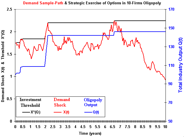
The figure below shows these features for a certain demand sample-path
X(t) in 10-firms oligopoly. When the demand rises at the threshold level all firms exercise options to expand capacity, increasing the aggregated industry output.

In this model, the firms' addition of capacity is proportional to the difference between the demand shock X(t) and the threshold level X*(Q(t)), if positive. In case of the demand below the threshold X*, no investment is performed (and no exit as well).
In the Grenadier's model the firms are equals, so that in 10-firms oligopoly case each firm adds 1/10 of the new capacity Q(t) - Q(t - dt) in case of positive shock at t, if X(t) > X*(Q(t - dt)).
The figure above also shows that, for this specific sample-path, after the year 8 the demand drops to levels well below the demand level at t = 0, but the total industry output remains (so that the prices drops). This model does not consider reduction of industry output due to low demand state. A possible improvement in the model is to consider other options like the option to temporary stopping (at cost) and the option to exit.
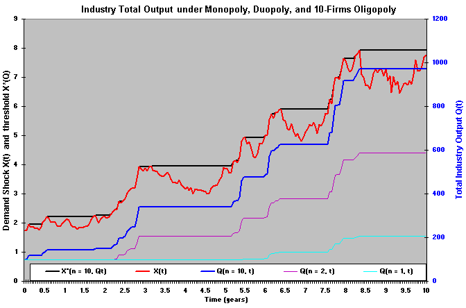
The figure below shows for one demand evolution sample-path, that the industry total output Q(t) is much higher for the 10-firms oligopoly (n = 10) case than for duopoly (n = 2), which presents a higher industry output than the monopoly case (n = 1).

The figure above shows that, for the same demand evolution, after 10 years the oligopoly with 10 firms produce together near 1000 units, whereas the duopoly and monopoly produce near 600 and 200 units, respectively.
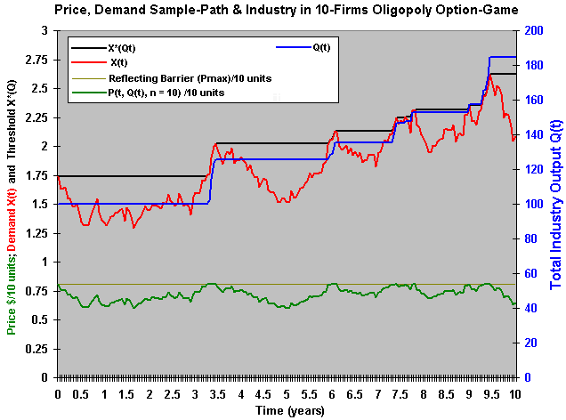
The figure below shows the evolution of the prices, considering the demand shock and the oligopoly addition of capacity. Note that there is an upper reflecting barrier at $ 0.8081/10 units, so that when exists a positive demand shock reaching this reflecting barrier, the oligopoly addition of capacity is sufficiently high to the prices either to remain at this level (if demand remains rising) or to be reflected-down. The figure below shows this feature for a certain demand sample-path.

Download the Excel spreadsheet simulation-oligopoly_equilibrium.xls (file with 291 KB), and see 4 charts
- including the 3 charts from the above figures. Press F9 in order to see new sample-paths with the
consequents results in terms of thresholds, industry production, prices, etc.
The non-registered version can be freely downloaded below and used for educational purposes:
![]() Download Excel file named simulation-oligopoly_equilibrium.xls
with 291 KB
Download Excel file named simulation-oligopoly_equilibrium.xls
with 291 KB
This spreadsheet is a component from the software pack Option-Games Suite. The registered version the sheet of calculus is non-protected and the registered reader can see the calculation details.
See how to register the real options software and the licence fees