For commodities and interest rates (and perhaps for exchange rates)
mean-reversion model has more economic logic than the geometric Brownian
model presented before.
Suppose that the petroleum prices P follow a geometric mean-reverting
process:
dP = h P (M - P) dt + s P dz
Where M is the long-run equilibrium level (or the long-run mean price
which the prices tend to revert); and h is the
speed of reversion.
The others terms have the same meaning of the geometric Brownian motion
(GBM) case, presented before.
In the financial-economics literature appear several different ways to model the mean-reversion process. This format of mean-reverting process was studied by Dixit & Pindyck (1994), and is also known as Geometric Ornstein-Uhlenbeck or Dixit & Pindyck Model.
The difference between a mean-reverting process and the GBM is the drift
term:
the drift is positive if the current price level P is lower than the
equilibrium level M, and negative if P > M.
In others words, the equilibrium level attracts the prices in its
direction. The analogy is with a spring: how more distant are the prices
away the equilibrium level, higher is the tendency to revert back the
level M.
The most basic mean-reversion model is the (arithmetic) Ornstein-Uhlenbeck model, which is discussed below in a specific topic. This name is due to the paper that first discussed this model, "On the Theory of Brownian Motion", by G.E. Uhlenbeck and L.S. Ornstein, in Physical Review vol.36, September 1930 (reprinted in N. Wax, eds., Selected Papers on Noise and Stochastic Processes, Dover Pub., 1954, pp.93-111).
As pointed out by Stroock (1993, p.220n), the authors "introduced this process in an attempt to reconcile some of the more disturbing properties of Wiener paths with physical reality". In real options this is also the motivation: people looking for a process with properties more adherent to economic reality, e.g., with demand and supply forces acting when the prices are far from a "more reasonable" equilibrium level.
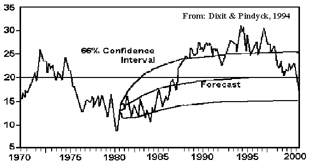
The following picture illustrates this stochastic process, showing one sample path, the 66% confidence interval, and the forecasted expected value (trend line in direction to the long-run equilibrium level).

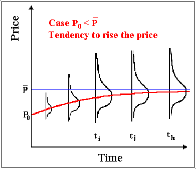
The Mean Reversion Process is a log-normal diffusion process, but with the variance growing not proportionally to the time interval. The variance grows in the beginning and after sometime stabilizes on certain value. The stabilization of the variance is due the spring like effect of the mean-reversion. The picture below illustrate this, for "low prices" case:

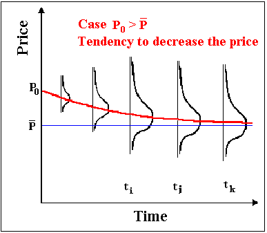
The picture below illustrate the mean-reversion for the "high prices" case:

The mean-reversion process has been considered the natural choice for
commodities. Basic microeconomics theory tells that, in the long run, the
price of a commodity ought to be tied to its long-run marginal production
cost or, "in case of a cartelized commodity like oil, the
long-run profit-maximizing price sought by cartel managers"
(Laughton & Jacoby, 1995, p.188).
In other words, although the oil prices have sensible short-term
oscillations, it tends to revert back to a "normal" long-term
equilibrium level.
Production cost varies largely across the countries, mainly due to the
geologic features, and most of the lower cost countries belong (or are
influenced) by the OPEC cartel.
Hence, even with a growing non-OPEC production, the OPEC role remains very
important in the production game of the petroleum industry. The large oil
prices rising in February-April 1999 is mainly due the articulation power
of OPEC (and its eventual allies) in reducing the production.
There are several evidence that oil prices are mean-reverting.
For example the econometric tests of D. Pilipovic (1998, table 4-9, p.78,
WTI petroleum).
Pindyck & Rubinfeld (1991, chapter 15) using a Dickey-Fuller unit root
test, rejected the random walk hypothesis for a very long time series
(more than 100 years).
But they point that the oil price reversion to a long-run equilibrium
level is likely to be slow.
Other important mean-reverting evidence comes from futures market, as
pointed out by Baker et al (1998, pp.124-127).
First, the term structure of futures prices are decreasing (toward the "normal"
long-run level, in backwardation) if the spot prices are "high",
and are increasing (in contango) if prices are "low".
Second, if the prices are random walk, the volatility in the futures
prices should equal the volatility of the spot price, but the data show
that spot prices are much more volatile than futures price. In both cases,
the mean-reverting model is much more consistent with the futures prices
data than random walk model. In addition, the econometric tests from
futures term structure performed by Bessembinder et al (1995, p.373-374)
also reveals strong mean-reversion for oil prices and agricultural
commodities (but weak reversion for precious metals and financial assets).
Sometimes is preferred work with the arithmetic process for the
logarithm of the stochastic variable, mainly for simulations and
parameters estimation, due the simplicity.
Suppose the petroleum (crude) price is P and let x = ln(P).
Consider that x follows the arithmetic Ornstein-Uhlenbeck process toward
an equilibrium level m:
dx = h (m - x) dt + s dz
The variable x has normal distribution, the expected value of x and the variance are shown below. The expected value equation is:
E[x(t)] = m + ( x(0) - m) exp(- h t) = x(0) exp(- h t) + m (1 - exp(- h t))
In the left format of the equation the interpretation is more clear: the
expect value will be an intermediate point between x(0) and the mean m,
weighted by a decay rate. The weights sum one.
There are two ways to found the above equation. The first, more rigourous,
through the stochastic integral format for the arithmetic
Ornstein-Uhlenbeck process (see below) and taking expectations
(and the Itô integral goes to zero).

The second way to get the same equation for the expected value, is simply by integrating directly the deterministic term of the arithmetic Ornstein-Uhlenbeck process dx/(m - x) = h dt.
The variance of the Normal distribution of the variable x at the instant t is:
VAR[xt] = [1 - exp(- 2 h t)] s 2/2h
See that there is a time decay term for the variance. For long time
horizon the variance of this process tends to s
2/2h.
So, unlike the Brownian motion the variance is bounded (not grows to
infinite).
This format ease the parameters estimation (see estimation below). Possibly due to this advantage, Schwartz ("The Stochastic Behavior of Commodity Prices: Implications for Valuation and Hedging", Journal of Finance, vol.52, n. 3, July 1997, pp.923-973, and with reference to an unpublished manuscript of Ross) used the following equation to represent the one-factor model of a mean-reverting commodity price (P):
dP = h (m - ln P) P dt + s P dz
Compared with the Dixit & Pindyck Model (DPM), the new thing here is
the term ln P in the equation of P, and instead M appear
m. By one side it seems less natural because investors have little feeling
about values expressed in logarithm, mainly for the equilibrium price or
long run mean.
But this model has the modeling advantage mentioned above.
Applying the Itô's Lemma for x = ln P, results:
dx = h* (m* - x) dt + s dz
Where:
m* = m - s2 /(2
h)
h* = h
By estimating m* and h*, it is easy to obtain the original model parameters.
The natural choice of a mean-reverting model for the commodity price (P) could be the DPM mean reverting model (because is more intuitive think about reversion to oil price long run mean price M, instead the long run mean of the logarithm of the price) repeated below:
dP = h P (M - P) dt + s P dz
The disadvantage feature of the DPM model is the logarithm transformation by the Itô's Lemma (of the x = ln P), because the corresponding parameters are function of P itself. For the equation of dx:
dx = h* (m* - x) dt + s dz
The parameters in this case are:
m* = ( M - s2 /(2
h)) ln P/P
h* = h P/(ln P)
Which depend on the price P level. Hence, this model format has the disadvantage that the logarithm transformation by the Itô's Lemma gets parameters that are not constant (function of P).
In practice, however, the estimation problem is not so critic because given that the parameters m* and h* are estimated, the parameters M and and h could be estimated as an average of a reasonable price interval (for example the case of oil prices, the range could be 10-30 $/bbl). The parameters variation normally is not too large with the prices levels.
What is the better model? A difficult answer because both have
advantages and weakness.
By the economic point of view, DPM model is clearer because works with
prices reverting to a long run level, instead reverting to a logarithm of
a mean . But the parameters are not constant (function of P).
The Schwartz-Ross model is less intuitive for the user but the parameters
are indepent of P and so is more modeler's friend.
DPM or Schwartz? The reader has the last word.
Parameters Estimation
The equation describing dx, the arithmetic Ornstein-Uhlenbeck equation presented above is a continuous time version of the first-order autoregressive process, AR(1), in discrete time (see Dixit & Pindyck, p.76; or Schwartz, 1997, footnote 15). It is the limiting case (Dt tends to zero) of the AR(1) process:
xt - xt - 1 = m (1 - e- h Dt) + (e- h Dt - 1) xt - 1 + et
Where e t is normally distributed with mean zero and standard deviation se, and:
se2 = [1 - exp(- 2 h)] s 2/2h
In order to estimate the parameters of mean-reversion, run the regression:
xt - xt - 1 = a + b xt - 1 + et
Calculate the parameters (it is easy to see why by looking the AR(1) equation):
m = -a/b ;
h = - ln(1 + b);

Where se is the standard
deviation from the regression (the last equation corrects a small typo in
Dixit & Pindyck).
The unit in the above equation is percentage by time unit, and of course
the time unit is the same time-series unit (if using monthly time-series,
it is % per month, etc.).
If we use monthly data and we want to obtain annual values for the
parameters, multiply the value of h, obtained
in the equation above, by 12; and multiply the value of
s obtained above by the square-root of 12,
etc.
One important distinction between random walk and stationary AR(1) processes: for the last one all the shocks are transitory, whereas for random walk all shocks are permanent.
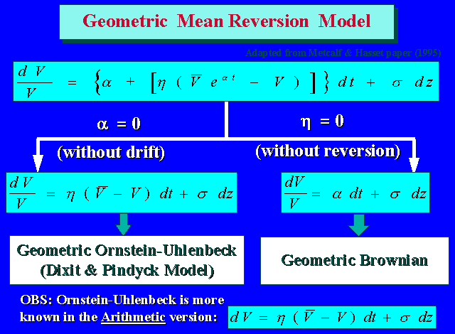
The figure below presents a combination of Geometric Brownian Motion (exponential drift) with mean-reverting model. This was adapted from Metcalf & Hasset (1995).

![]()
Other important type of stochastic process description for oil prices are the models with two and three factors.
The two-factor models, as in Gibson & Schwartz ("Stochastic Convenience Yield and the Pricing of Oil Contingent Claims" Journal of Finance, vol.45, no 3, July 1990, pp.959-976), generally uses GBM for spot oil prices and a stochastic mean-reverting convenience yield d. This additional factor corrects the main bias from the one-factor GBM model, becoming more consistent with the market data from the futures term structure.
The two stochastic processes equations are:
dP = (m - d) P dt + P sp dzp
dd = h (D - d) dt + sd dzd
Where D is the long run mean convenience
yield value, h is the speed of reversion of
the convenience yield. The others are as before.
These stochastic processes are correlated (positively in this case). The
equation is:
dzd dzp = r dt
Where r (- 1 to + 1) is the correlation factor for these processes.
Schwartz (1997a, p.943, Table IX) finds strong correlation between the oil spot price and the convenience yield (+0.915 for 259 samples and + 0.809 for other 163 samples).
The futures equation for the oil prices in this model is:
F(P, d, t) = P exp{- d [(1 - e- h t )/ h] + A(t) }
Where A(t) depends of the time and the parameters of the process, but do not depend neither on the spot price P nor the convenience yield d.
The three-factor model is presented in one article of Schwartz (
"The Stochastic Behavior of Commodity Prices: Implications for
Valuation and Hedging" Journal of Finance, vol.52/ 3, July
1997, see pp.929-931), allowing the interest rate to be the third
stochastic factor, also modeled as mean-reverting.
The three stochastic processes are correlated and was performed a complex
empirical job (using Kalman filter) to estimate several parameters of
these processes.
He compares it with the one and two-factor models.
Schwartz (1997a, p.943, Table IX) finds that the correlation between spot price and interest rate (r) were slight negative (- 0.0293 and - 0.0057), whereas between d and r seem to be independent (- 0.0039 and + 0.0399).
![]()