 4) Mean Reversion with Jumps Models.
 4) Mean Reversion with Jumps Models.
For oil prices and perhaps for others commodities, interest rates, and exchange rates, an interesting and perhaps the best
stochastic process is a Poisson-Gaussian model of mean-reversion with jumps.
This model has more economic logic and considers large variation of the underlying variable due the
arrival of abnormal rare news.
For an introduction to the mixed Poisson-Gaussian (or jump-diffusion) process, see my section in the appendix on Poisson-Gaussian Processes.
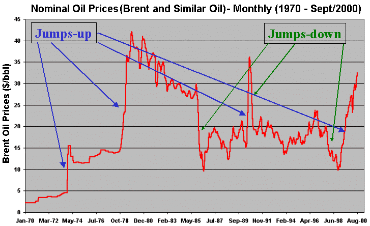
The figure below shows the oil prices (Brent and similar oils) since 1970, which exhibit sometimes jumps-up and jumps-down, linked to abnormal shock either on production (most cases) or in demand:

The jump-diffusion model links the prices changes to arrival of information. There are two types of information, the normal news with smooth variation in the oil prices, and the abnormal news, with jumps in the prices. The smooth variation is modeled by a mean-reversion process (continuous process), whereas the jumps are modeled with a Poisson process (discrete time process).
The Poisson process is a counting process in which interarrival times of sucessive jumps are independently and identically distributed (i.i.d.) exponential random variables.
Suppose that the petroleum prices P follow a geometric mean-reverting with jumps process:
dP = h P (M - P) dt + s P dz + P dq
Where M is the long-run equilibrium level (or the long-run mean price which the prices tend to revert); h is the speed of reversion; dq is the Poisson (jump) term; and the other terms have the same meaning presented before.
The Poisson term dq values zero most of time, but with frequency l, it assume a value causing a jump on the underlying variable.
dq = 0 . . . . . . . with probability 1 - l dt
dq = F - 1 . . . . . . . with probability l dt
The usual and practical assumption is that the Wiener (dz) and Poisson (dq) processes are not correlated.
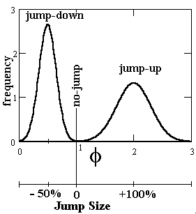
The jump size/direction can be random. In the above equation F is the jump size probability distribution. Given a jump, the expected jump size is k = E[ F - 1].
The figure below show a random jump sizes, for both cases, jump-up and jump-down.

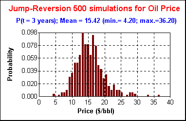
A possible price distribution for a future price, drawing from a jump-reversion simulation is:

Due the jumps, the oil prices can reach very lower (under 5) or very high (above 36) values. But most values are near the mean due the reversion force. In the above case the long run mean was considered for a heavy oil, with a level of 15 $/bbl.
A model with practical advantages, sometimes used (see Dias & Rocha, 1998), is the compensated Poisson version for geometric mean-reversion with jumps process:
dP/P = [h (M - P) - l k ] dt + s dz + dq
There is an additional term in the drift, - l k,
the compensation term.
The compensated Poisson process allows that the expected value of dP/P to be
independent of the jump parameters.
Neftci book (1996, p.115) states the simple principle: If somehow a stochastic process is
not a martingale, then by subtracting a proper "mean" it can be transformed into a
martingale.
A Poisson process Nt is a counting process, so increase with the time and cannot
be a martingale, but a compensated Poisson process
(N*t = Nt - lt) will be a martingale (Neftci, 1996, p.116; Neftci, 2000, p.179).
In our Poisson process case, E(dq) = k ldt, so we get the
compensation term above.
The advantage of jump-reversion process is that describes better the reality by both point of view, economic (microeconomic logic) and by the statistical time-series (explaining the skewness, fatter tails, abnormal movements of oil prices). But there is a cost. The two problems with jump-diffusion processes are: the impossibility to build a riskless portfolio; and the difficulty with parameters estimative.
The first important problem when considering jumps in the option valuation is that is impossible to build a perfect hedge. So, in general is not possible to build a riskless portfolio as in Black-Scholes-Merton contingent claims approach.
The second problem is the job of the parameters estimative:
There are several parameters to estimate, and in general is hard to estimate the law (and the parameters)
for the jump-size distribution F (mainly because we are interested in
large but rare jumps, so there is a lack of data to estimate the jump-size parameters).
The two general approaches to estimate parameters in options models are:
(1) statistical approach, from historical data; and
(2) implied approach from the market data, that is, from the options prices (as is performed with
implied volatility, is possible to get implied jump-arrival and so on).
For the statistical approach there are several methods, from the Classical School using Kalman
Filter; to the Bayesian School using Markov Chain Monte Carlo.
Researchers working with jump-diffusions processes, such us Prof. Das and Prof. Bates, has been
using several approaches to joint estimate of parameters in jump-diffusion processes.
Others authors (see for example Zein, 1999, and Dias & Rocha, 1998/9) take a more practical
approach and separated the parameters estimative from these two independent processes. By taking out
of the sample the jumps, you get a time-series to estimate the diffusion parameters (like volatility, and in
case of mean-reversion, the long-run mean and the reversion speed) as showed before. The out sample
data (the jumps) is counted to determine the jump frequency (l).
In this approach, is necessary to define jump in the data. For example, in a monthly data, jump is when the
variation in a month is equal or higher 30% (jump-up) or equal or less than
- 20% (jump-down).
The mean size of the jump and the dispersion of this size could be inferred with the data, but as the
number of jump samples is too small, a practical feeling about the jump-size is also acceptable.
A sensitivity analysis can be performed to check how critical is the jump-size distribution
parameters assumption in our specific problem. In some cases (as in Dias & Rocha, 1999, see the
page of Extendible Options Using Mean-Reversion + Jumps), are not
important the standard deviations of the jump-ups and jump-downs, whereas the jump arrival frequency
l has a more relevant impact on real options valuation.
Even the use of more subjective "reasonable parameters values" with a better mapping
as a jump-reversion model may perform better than an "easier parameter estimation", which
not capture some important possibilities of the probabilistic mapping.
The conclusion is that even with these practical problems, the better mapping of jump-reversion for
oil prices is a sufficient advantage to go ahead with this model.
These practical problems with the passage of time will become
less important: with new econometrics approaches, in a near future the parameters estimative problem
will become a dominated task, and interactive softwares easily will find the parameters for a given
time-series data and specifying the desired stochastic model!
Suppose the petroleum (crude) price is P and let x = ln(P). Consider that x follows the arithmetic mean-reversion with jumps:
dx = d[ln(P)] = [h [m - ln(P)] - l k ] dt + s dz + dq
Where m = ln(M) is the long-run mean of the logarithm of the prices.
The expected value of the logarithm of the petroleum price in this model is:
E[ln(P)] = ln(M) + {[ln(P0) - ln(M)] exp(- [ln(2) t ]/H)}
Where the half-life H = [ln(2)]/h
Now suppose the following arithmetic jump-reversion, without the compensation term:
dx = d[ln(P)] = h [m - ln(P)] dt + s dz + F dq
Where F is distribution of jump sizes.
The mean jump size is k = E[F].
The Poisson variable dq values 0 most of time and 1 sometimes (= 1 with probability
l dt).
The first probabilistic moment, the mean of this process, is:
E(x) = E[Ln(P)] = (m + (l k H/ln(2))) x (1 - exp(- ln(2) t/H)) + [ln(P0) exp(- ln(2) t/H) ]
If the average jump is zero, that is k = 0, using this result in the equation above you get the same result of the compensated Poisson case.
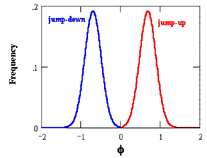
One possible case of jump size with zero mean is shown in the following picture that illustrate a possible distribution for the jump size:

In order to find the variance of the process is necessary to solve a PDE
(partial differential equation) for the probability density function (Kolmogorov equation).
Das (1998) presented a solution for this process (he used for interest rates, but the adaptation for
oil prices is direct). The variance of the distribution for x, is its second moment
(M2)
less the square of the first moment, that is
Var(x) = M2 - [E(x)]2.
In other words, the variance is given by:

Note that:
![]()
In order to find out this expected value is necessary to solve numerically the following integral:

Where f is the jump size and f(f ) is probability distribution of the jump size.
The higher probabilistic moments from the distributions generated by jump-diffusion processes
define caracteristics like the typical fat tails of the distribution.
Unlike the normal distribution, the distribution of the returns generated by the
jump-diffusion process is assymetric with fatter tails.
Assets returns following jump-diffusion, generally
presents a positive skewness.
Skewness is a measure of symmetry (skewness is 0 for symmetric distributions like the normal one) and
positive skewness means distribution with long positive tails (skewed to the right).
Skewness is related to the third moment (M3).
A dimensionless measure is the ratio:
M3 / s3
The skewness for the jump-reversion process presented is the following equation:


Kurtosis shows how flat or peaked the distribution is.
It is a measure of the distribution shape.
Higher peaked is the distribution, higher is the kurtosis.
Kurtosis is related to the fourth moment (M4).
A dimensionless Kurtosis coeficient is the ratio:
M4 / s4.
The normal distribution has a kurtosis coeficient equal 3.
For the equations and discussions of the higher probabilistic moments of the jump-diffusion
processes and the density of the distribution, see Das
("Poisson-Gaussian Processes and the Bond Markets", NBER Paper #6631, 1998)
With the expected value, the variance, and higher moments, the forecasting and
risk mapping jobs can be performed.
![]()