Answer: Real options theory provides new insights on this very interesting and important application.
A large Petrobras-PUC research on this topic is finishing in 2004.
The aim of this research was the comparison of alternatives of oilfield development,
alternatives of investment in information, alternatives with option to
expand, etc., before commit a large investment in an offshore oilfield
development. The project topic covered in this FAQ finished in 2003, with a C++ software and a paper by Dias & Rocha & Teixeira (2003), submitted to publication.
Let us analyze the case of mutually exclusive alternatives to develop an oilfield. One simple model is presented by Dixit: "Choosing Among Alternative Discrete Investment Projects Under Uncertainty". Economic Letters, vol.41, 1993, pp.265-288.
This model is summarized below, with a little adaptation using the
concept of economic quality of a developed reserve(q).
If the oil price values P and one barrel of reserve values V, the quality
q = V/P. Here the normalized (by B) net present value NPV/B = q P - D,
where B is the reserve volume (number of barrels) and D is the normalized (by B) development cost (in present value).
OBS: In more recent papers I call V = q P B, but in this FAQ the notation is V = q P because we are working with normalized values ($/bbl) instead $.
The alternatives have different investment costs. Higher investment alternatives have benefit of faster production (more wells and/or higher processing facilities capacity) and/or lower operational costs. What is the optimal capital intensity under uncertainty?
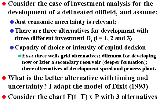
First, let us see the best decision at the expiration. The picture below illustrates this case:
Higher quality q means higher inclination in the chart above.
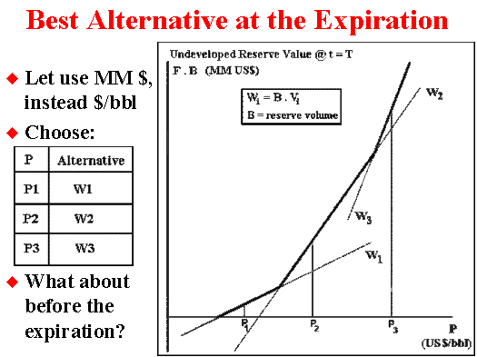
Before the expiration the analysis is a bit more complex. One
alternative alone can be "deep-in-the-money", but the existence
of other alternatives can change this, and the manager can wait and
eventually to invest in a larger scale alternative.
The picture below shows this case.
The alternative 1 could justify an earlier investment if the inclination
(the reserve quality) become a bit more inclined.
Other important point is: with passage of time, the options curve move
down and for a region of prices, the option curve of alternative 2 can be
below the option curve of the alternative 1, so that is possible to choose
an earlier exercise of alternative 1 for prices at or above the P1*
and lower than the intersection of the payoffs from alternatives 1 and 2.
It is easy to get the curves for the option alternatives with
spreadsheets like Timing. To compare, superpose the option curves and look for the higher one. With this practical approach we can see some special cases not addressed before by Dixit (1993). Even being an approximation (see below why), the numerical error on the value of the option is very small so that it possible to see that in most cases there is an intermediate waiting region between the exercise of alternatives 2 and 3. So that for P > P*2, we can see a region that the
option value of waiting (F3) is higher than both NPV2
and NPV3.
Motived with this somelike surprising experimental early result, in 2000 were started two projects between PUC and Petrobras - from the Pravap-14 research projects portfolio, which confirmed this hypothesis. One
Pravap-14 project was a more flexible and general determination of the
optimal rules regions by using genetic algorithms (developed with
Electrical Engineering Department). The other Pravap-14 project was more
rigorous (but specific for simpler cases) using the traditional differential
equation approach (developed with Industrial Engineering Department).
Both used finite-lived options. In year 2002 we started the second phase
of both projects, adding other realistic details with more complex issues.
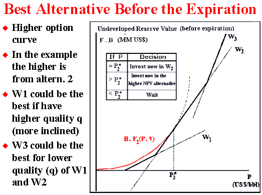
By using a C++ PRAVAP-14 software developed at Industrial Engineering
Department (PUC-Rio), it is possible to get the following thresholds chart
showed below (and presented at MIT Seminar on Real Options, May 2002).
Working independently and with perpetual options, Décamps & Mariotti & Villeneuve (2003) proved mathematically that the waiting region around the point of indifference between NPV2 and NPV3 always occurs (non-empty region) if sometimes is optimal to invest in alternative 2. They showed that if "investment in the smaller scale project is sometimes optimal, ... the optimal investment region is dichotomous.". In their proposition 3.2, they show that the indifference point where NPV2 = NPV3 does not belong to the exercise region. They proved with help of the sophisticated concept of local time for the continuous semimartingale P applied at this indifference point. Before this paper, I was thinking that the Dixit's (1993) claim even not being typical could be possible. But they proved that it cannot be possible.
Probably the conclusion from Décamps & Mariotti &
Villeneuve (2003) is even more general, being also true for finite-lived
options except at the expiration.
I thank to Professor Thomas Mariotti for letting me know about this paper
and for the nice discussion.
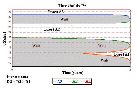
With this new insight in mind, we can correct the Dixit's option
value chart by setting a case that always occurs in the figure below
(analogous to Figure 1 from Décamps & Mariotti &
Villeneuve, 2003):
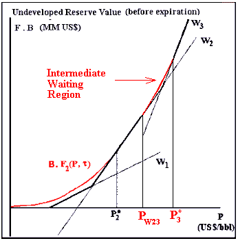
In the above figure, the option curve (red line) in the superior part of
this figure (between PW23 and P*3) is the
intermediate waiting region. Décamps & Mariotti &
Villeneuve (2003) showed that this region always exists (if sometimes is
optimal exercise alternative 2, as occurs in the figure).
Numerically the error can be small if exercising the option (higher NPV as
suggested by Dixit in 1993) rather than waiting in this intermediate
optimal waiting region. So, even not being correct, the error using the
Dixit's insight can be small in practice. However, the size of the waiting
interval (between PW23 and P*3) can be a large
range.
The full results from the Pravap-14 project (including cases with mean reversion) is reported in a paper by Dias & Rocha & Teixeira (2003), submitted to publication.
![]()