
1) Timing 2.0 Results, Charts, and New Features
. . . . . . . . . . What Is New in the 2.0
Version?
4) Timing Variants: Timing for Business Model and Timing for Rigid Cash-Flow Model
How to register software and licence fees.

This Excel application performs the real options analysis for an
opportunity to invest in a project, which is view as a finite lived
American call (real) option, with time to expiration T established by
legal terms (as in petroleum upstream) or by an estimative of expected
time for competition entry (Kester, 1984).
The operating project value V is the underlying asset of our real options
problem. The real option value F is the value of the right (but not
obligation) to invest in the project until a certain limit date. The
project value is uncertain and follows a geometric Brownian motion.
The main results from this application runs instantaneously (less than 1
second) in Pentium computers, only Monte Carlo simulations can take more
time (seconds or even some minutes) depending of the number of simulations
(the required precision for some outputs).
The main features of this applicative are:
There are two charts which are updated automatically when you change
the value from the parameters:
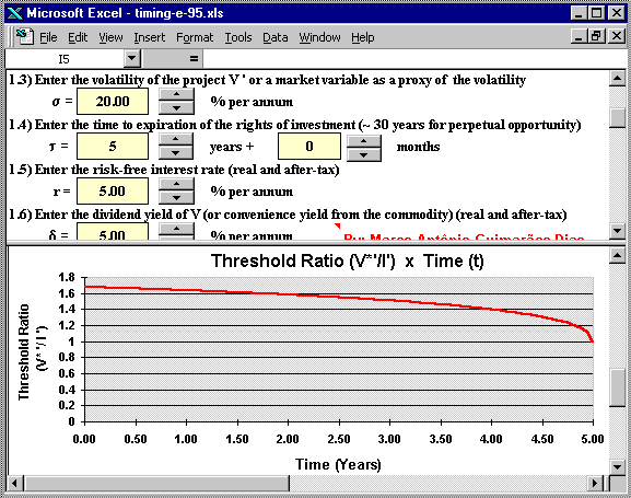
Real Option value chart and Threshold chart. The threshold chart shows the optimal investment option exercise curve along the time, named free-boundary by the mathematicians.
Using spinners to change the parameters, you can see (like an Excel "movie")
the lines in the charts moving.
In order to do this, I divided the Excel window into two panels: in the
upper panel you can change parameters (by clicking repeatedly on the
spinners) and in the lower panel you see the chart lines moving due to the
parameters variation.
For the option and the early exercise threshold calculus in this new Timing version, I use the better analytical approximation due to Bjerksund & Stensland ("Closed-Form Approximation of American Options", Scandinavian Journal of Management, vol.9, 1993, pp.87-99). The resulting values are very good approximation for real options applications.
Think that the project is not deep in the money and is better to wait. What is the probability of the investment option to be exercised, until a certain time to expiration T? Conditional to the the option exercise, what is the expected option exercise time (also known as expected first hitting time). The answers to these questions are important inputs to analyze the multi-year investment budget of the whole portfolio of projects.
These estimates are performed using both a traditional Monte Carlo Simulation and a Hybrid Quasi-Monte Carlo Simulation. See more about simulation in the page about Monte Carlo Simulation and in the page on Quasi-Monte Carlo Simulation.
The expected first hitting time is the expected time spent for a
stochastic variable to reach a certain value.
For example: suppose the current oil price is 18 US$/bbl and suppose an
arbitrary superior price level of US$ 21/bbl. If the oil prices follow a
geometric Brownian motion, what is the expected time for the oil prices to
reach the US$ 21/bbl level? The answer is the mentioned expected first
hitting time for a variable (oil price) that follows a Brownian motion
(others stochastic processes are possible, too).
For a formal definition, real options applications, discussion of hitting times probabilities and equations, brief bibliographical review, others theoretical issues, and how to use the Excel
program features related to the expected
first hitting time, click here.
The new Timing version has many important differences compared with the older Timing version:
First, now it is using VBA (Visual Basic for Applications) macros
and user-defined functions. By using VBA, the spreadsheet size is
lower and faster than the previous Timing version. In addition, it permits
to perform a Monte Carlo simulation by using macros.
The VBA code is password protected, but the references given here permit
the interested reader to access the sources (formulas and algorithm codes
in some cases) and build a code by him/herself, or even to check the
results obtained with Timing.
Second, this version uses a better analytical approximation due to
Bjerksund & Stensland ("Closed-Form Approximation of American
Options", Scandinavian Journal of Management, vol.9, 1993,
pp.87-99), replacing the popular Barone-Adesi & Whaley's analytical
approximation used in the previous version of the Timing Suite.
According the Haug's book (The Complete Guide to Option Pricing
Formulas, McGraw-Hill, 1998), which this analytical approximation is
detailed in formulas and a VBA code, Bjerksund & Stensland (1993) is
more accurate than the more popular Barone-Adesi & Whaley (1987) for
long term options. This is exactly the general case of real options and so
Bjerksund & Stensland (1993) is used to calculate both the real
option value and the optimal decision rule.
Third, it calculates the probability of option exercise and, conditional to the the option exercise, the conditional expected time of option exercise, that is, the expected first hitting time for the simulated sample paths to reach the threshold curve conditional to option exercise occurrence. The calculus can be performed through a traditional Monte Carlo simulation or, even better, by using the more accurate Hybrid Quasi-Monte Carlo Simulation. Both simulation alternatives are available for the user comparison.
In this applicative I divided the Excel window into two panels: in the upper panel you can change parameters (by clicking repeated on the spinners) and in the lower panel you see the new results (of real options value or the optimal decision rule) or can see the chart lines moving (as a "movie") due the parameters variation.
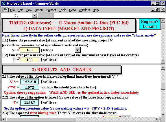
The pictures below show the Timing screens.
The first Timing screen shows the upper panel as data input entry and
the lower panel as the solutions mainly for option value and threshold.
In the bottom part appears the facilities for calculus of the probability
of option exercise and the expected time of option exercise, with both
hybrid Quasi-Monte Carlo Simulation (better) and the traditional Monte
Carlo Simulation.
As mentioned before, there are two charts that are updated automatically
when you change the value of the parameters in the upper panel:
The option value chart and the threshold chart (the
free-boundary).
The second picture (below) shows the Excel program screen with upper panel displaying the input data with spinners facilities and the lower panel exhibiting the free-boundary chart (the threshold for immediate investment chart).
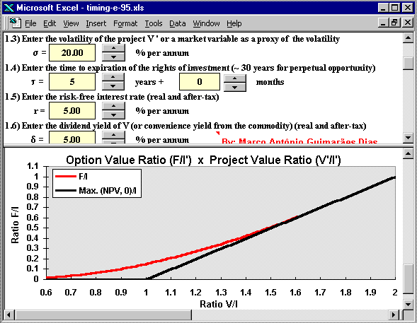
(c) the third picture (below) shows the Excel program screen with upper
panel presenting the input data with spinners facilities and the lower
panel exhibiting the option value chart.
In this spreadsheet you can remove the freeze panels in menu "Window", but is far
more interesting to see the results changing in the lower panel due the
changing of the parameters in the upper panel.
Another Excel tip: in order to gain visual area (mainly if you use low video resolution as 800 x 600 or 640 x 480), remove the toolbars (menu "View/Toolbars") and others Excel facilities in the menu "Tools/Options/View" (formula bar, status bar, row & column headers, and sheet tabs).
Next are showed the Timing version 2.0 facilities to calculate the conditional expected first hitting time and the probability of the option to be exercised, for finite lived options, using the Monte Carlo approach. The figure below illustrates these facilities in the software "Timing":
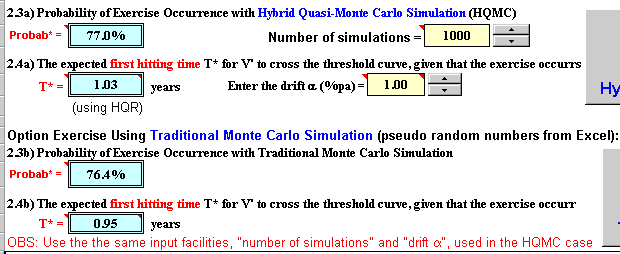
In the above figure we see that there are two alternatives to calculate the conditional expected hitting time and the probability of exercise. The first alternative is by using the more precise hybrid quasi-random numbers, see the webpage on the quasi-Monte Carlo and the section with hybrid quasi-random sample-paths. The second one is by using the traditional pseudo-random numbers (from Excel).
Note also in the above figure that is required the drift in order to calculate both the expected first hitting time and the probability of option exercise. Recall from the webpage on expected first hitting time that, although in option pricing generally we don't need to know the drift, this is not true for the case of the expected first hitting time calculus. Some options properties like the first hitting time do depend of the drift (expected growth rate) of the underlying stochastic variable. So, in this Excel application you need to set the drift.
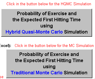
In the last picture, at the extreme right side the simulation buttons are cut. The figure below shows the two buttons, one for quasi-Monte Carlo simulation and the other for the traditional Monte Carlo simulation.
The file below is the Excel 97 for Windows spreadsheet named Timing, a shareware with full capability.
DISCLAIMER: The usual disclaimer applies for this Excel application. I'm not responsible for any consequences from this software use.
In order to download the shareware file, click the link below (Netscape users recommended to download the compressed version):
![]() Download Timing
(shareware), Compressed Excel file named timing-e-97-vba-hqr.zip
with 629 KB
Download Timing
(shareware), Compressed Excel file named timing-e-97-vba-hqr.zip
with 629 KB
![]() Alternative Download Timing
(shareware), Non-Compressed Excel file named timing-e-97-vba-hqr.xls
with 693 KB
Alternative Download Timing
(shareware), Non-Compressed Excel file named timing-e-97-vba-hqr.xls
with 693 KB
TIMING is shareware (but with full capabilities): if you like
it you need to register. See how to register
software and licence fees.
Any question, send me E-mail: marcoagd@pobox.com
People without Excel license can view and calculate (but not save) with the FREEware Excel Viewer, which can be found out in the Microsoft's Site
Registered users of Timing version 2.0 get for free full-functional versions of the new two variants of Timing:
Timing for Business Model and Timing for Rigid Cash-Flow Model.
These software variants are best described in the webpage on Linear and Nonlinear Models for the Underlying Asset V(P) and the NPV Equation. I recommend strongly that the reader visits that webpage for details related with these models, including charts, comparative tables, demonstrations, etc.
But here I set a very short description and the download links.
In short, these variants permits to work directly with the commodity price P as the basic stochastic variable, instead the value of the project V.
In order to work with the oil (or other commodity) price, are established equations linking the operating project value V with the commodity price P, that is the function V(P).
The Business Model uses the simple proportional equation, that is, V is proportional to P in the equation below:
V = q B P
Where B is a scale factor, in case of petroleum project is the reserve volume (number of barrels in the oilfield) and q is the project quality factor that in petroleum is named the economic quality of reserve (takes into account the discounting effect and the operational cost, among others effects).
The name "Business Model" is because this equation gives the value of a developed reserve in reserve transactions: q . P is the value of one barrel of reserve, used as reference in reserves markets. Multiplying this value of one barrel by the number of barrels gives the value of the transaction.
The Rigid Cash Flow Model is relies more heavily in the project cash-flow equations. Without operational options, and for the regime of concessions in the petroleum case, the value of the project is a linear function between V and P, but not proportional as in the previous case.
This linear equation is:
V = q' B P - C
Where C is the present value of part of the operational costs (fixed OC), whereas the other terms have similar meaning compared with the previous model.
The Excel spreadsheet below, shareware available to download, is the Timing Version Business Model, which calculates real options, threshold, probability of exercise, and expected first-hitting time conditional to exercise, using the "Business Model".
![]() Download the Excel spreadsheet
Timing Version Business Model
(timing-business_model-vba-hqr.xls), with 702 KB
Download the Excel spreadsheet
Timing Version Business Model
(timing-business_model-vba-hqr.xls), with 702 KB
![]() Or
download the compressed (.zip) version of this spreadsheet
Timing Version Business Model
(timing-business_model-vba-hqr.zip), with 636 KB
Or
download the compressed (.zip) version of this spreadsheet
Timing Version Business Model
(timing-business_model-vba-hqr.zip), with 636 KB
The only limitation of this spreadsheet compared with the registered version, is that some inputs are fixed in this non-registered version. The fixed inputs are: Initial oil price; investment cost; risk-free interest rate; and dividend yield (or convenience yield). Registered users can freely change any input.
The Excel spreadsheet below, shareware available to download, is the Timing Version Rigid Cash Flow Model, which calculates real options, threshold, probability of exercise, and expected first-hitting time conditional to exercise, using the "Rigid Cash Flow Model". It considers that the (long run expectation on) oil prices follows a geometric Brownian motion (GBM).
![]() Download the Excel spreadsheet Timing
Version Rigid Cash Flow Model (timing-rcf_model-vba-hqr.xls), with
703 KB
Download the Excel spreadsheet Timing
Version Rigid Cash Flow Model (timing-rcf_model-vba-hqr.xls), with
703 KB
![]() Or
download the compressed (.zip) version of this spreadsheet
Timing Version Rigid Cash Flow
Model (timing-rcf_model-vba-hqr.zip), with 637 KB
Or
download the compressed (.zip) version of this spreadsheet
Timing Version Rigid Cash Flow
Model (timing-rcf_model-vba-hqr.zip), with 637 KB
The only limitation of this spreadsheet compared with the registered version, is that some inputs are fixed in this non-registered version. The fixed inputs are: Initial oil price; investment cost; operational cost factor; risk-free interest rate; and dividend yield (or convenience yield). Registered users can freely change any input.