FAQ Number 14

How to Combine Technical and Market Uncertainties into a Dynamic Real Options Model?

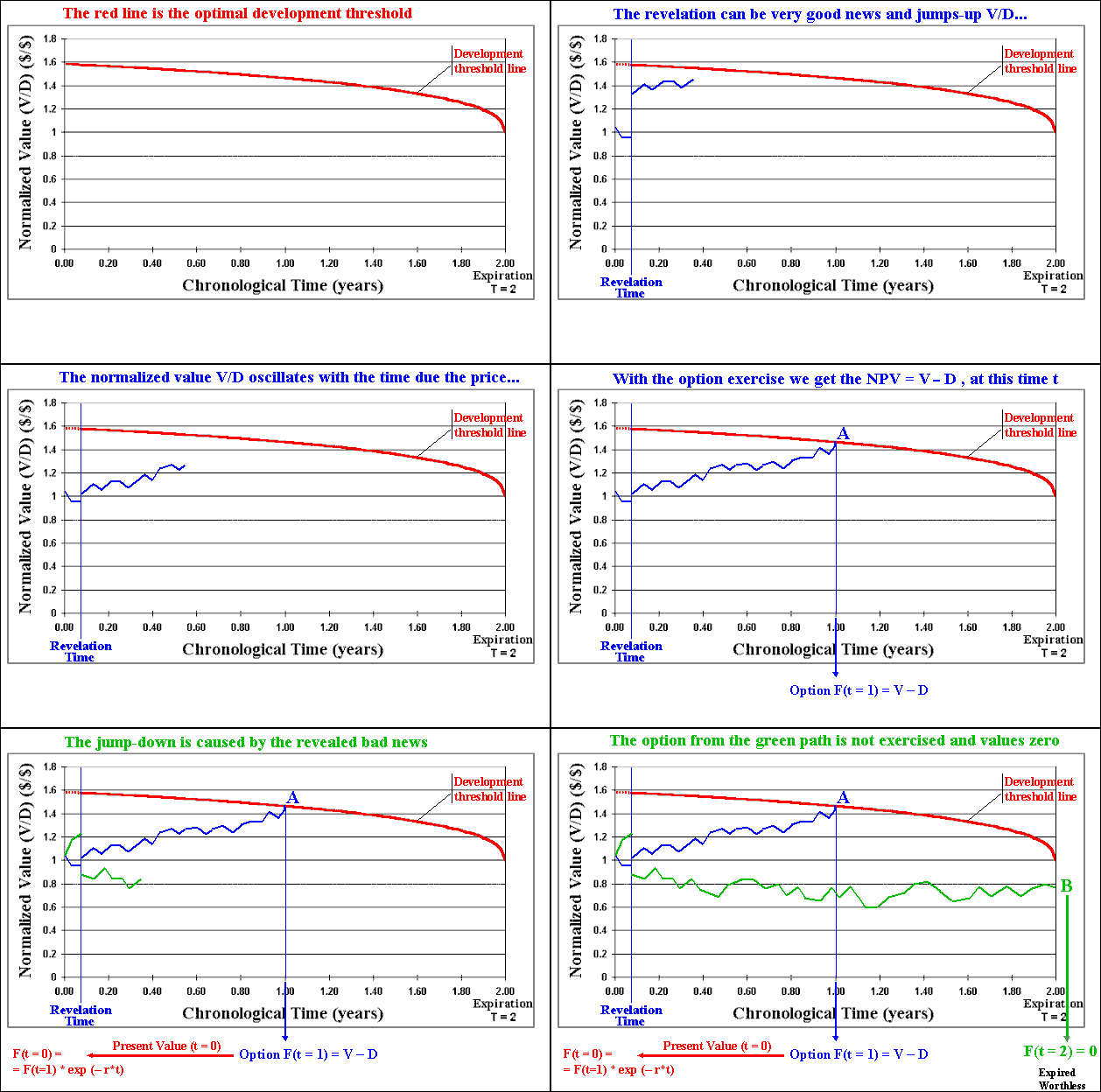
Answer: A simple way is by using the concept of revelation distribution into a Monte Carlo simulation framework..

The idea - presented in details in my paper on this subject, is summarized below (see also the animations after the topics):

1. We shall invest in information in order to learn about a variable X with technical uncertainty. We can get good or bad news. Considering a continuum of possible news, almost surely we will revise the expectations about the variables with technical uncertainty. For example, the uncertainties about the existence, the volume, and the quality of an oil reserve.
   
2. The revision of expectations is a function of the knowledge revealed by the investment in information, e.g., by drilling an appraisal well the reserve volume can increase or decrease depending on this well outcome. In technical terms, there is a distribution of conditional expectations E[X | Inf], where the conditioning is the new information revealed. I use the name revelation distribution to the distribution of conditional expectations.
   This distribution is used into the Monte Carlo framework and it has nice properties (click here for the propositions about the mean, the variance, the limit, and the martingale properties of the revelation distribution).
   Why conditional expectations? Click here.
3. In the dynamic framework, the revision of expectations at the information revelation causes a jump in the value of our project (and/or in the value of our investment in development). The size of this jump is drawn from the revelation distribution in the Monte Carlo simulation.
4. Imagine our payoff function is the development net present value (NPV), which is the difference (in present values) between the value of the operating project (V) and the development investment (D), so that NPV = V - D. That is, in case of exercise of the real option we get the NPV. Consider that V is function of a market variable P (e.g., the oil price) and of two technical variables: the volume (B) and the quality (q) of the oil reserve, which are uncertain. In addition, the optimal investment level depends on the expected reserve volume.
   So, the values V(P, B, q) and D(B) are revised at the information revelation instant due to the jumps in B and q (drawn from their revelation distributions), and V is revised continually along the time because the market variable P changes continually along the time according the assumed stochastic process for P. Here we assume that P follows a geometric Brownian motion (GBM) for simplicity: to take computational advantage using the homogeneity of the threshold curve (see below) we will work with the normalized value of the underlying asset V, i.e., V/D.
   
5. The animation below illustrates the valuation process for two sample paths. At the revelation time we have jumps in V/D because both are function of the technical variables B and q. The jumps in B and q are drawn from the revelation distributions.
   With the revised value V/D we proceed as usual in real options: we need to know if the option is "deep-in-the-money", i.e., if is optimal the immediate exercise. In order to do this we use the threshold curve (V/D)* showed in red below. If V/D >= (V/D)* at the time t, we exercise the option. Otherwise we "wait and see". Recall that the threshold curve is function of the risk-neutral stochastic process parameters, and using the GBM the threshold is homogeneous so that we can use the normalization (V/D)*.
   Let us see the animation to understand better the framework.

The animation below illustrates the methodology, which can be performed with the software Timing with Dynamic Value of Information. This chart of the normalized value of project V/D with the time, presents an example with time to expiration of two years and a time-to-learn of one month.

After N (hundreds or thousands) of sample paths we sum the options values obtained in each path (a lot of zeros and a lot of positive values) and divide by the number of simulations N. By subtracting the cost of the information, we finally get the real option value considering the investment in information and both technical and market uncertainties in a dynamic framework.

Note that we can perform the same calculus for several different alternatives of investment in information. In this framework, we can consider that the learning alternatives have different costs, different time-to-learn, and different benefits (captured mainly by the revelation distributions).
The framework is dynamic because consider the factor time: time-to-learn, time-to-expiration, and the continuous-time stochastic process for P. Our decision rule (V/D)* also depends on the time (because the option is finite-lived).

For additional information, see the page on Technical Uncertainty, Investment in Information, Information Revelation, and Revelation Distribution and the page on the software Timing with Dynamic Value of Information.

The Four Propositions for the Revelation Distribution:

1. Full Revelation Proposition: For the full revelation case, the revelation distribution is equal to the unconditional (prior) distribution.
   .
2. Mean of Revelation Distribution Proposition: The expected value for the revelation distribution is equal the expected value of the original (prior) technical parameter distribution.
   E[R_X] = E[X]
   .
3. Variance of Revelation Distribution Proposition: the variance of the revelation distribution is equal to the expected reduction of variance induced by the new information.
   Var[R_X] = Var[X] - E[Var{X | I }]
   .
4. Revelation Distributions as Martingales Proposition: In a sequential investment in information setting, the associated sequential revelation distributions {R_X,1, R_X,2, R_X,3, …} are event-driven martingales. In short, ex-ante these random variables have the same mean.

The first proposition is trivial - but very important as the limiting of a learning process, and it draws directly from the definition of prior distribution. The others three propositions are demonstrated in the paper appendixes
The second proposition is just an application of the law of iterated expectations. The third proposition is the central proposition because captures the revelation power of one investment in information, that is, the capacity of a learning process to reduce the uncertainty, which is directly linked to the revelation distribution variance. The last proposition helps the evaluation of different plans of sequential investment in information, permitting the application of martingale tools that is a well developed branch in probability and stochastic processes.

With the reasonable assumption that the prior distribution has finite mean and variance, Proposition 1 tells that even with infinite quantity of information, the variance of revelation distribution is bounded. This contrasts strongly with some real options papers that model technical uncertainty using Brownian motion, which the variance is unbounded and grows with the simple passage of time, which is also inadequate - this distribution changes only when new relevant information is revealed through investment in information.
About the last point, the figure below illustrates the difference of a continuous-time stochastic process (from a market variable like the oil price) and the evolution of a technical uncertainty (e.g., the reserve volume B). The figure shows one typical sample-path in each case along the time. The market variable changes with the simple passage of the time because every day investors expectations on the supply and demand are tested in the market, whereas the expected volume of a reserve changes only if new relevant information arrives from a new investment in information (in some cases due to new technology, but in most application it is even more dispersed in discrete points along the time).

Hence, the technical uncertainty evolves in discrete-time fashion and in most cases is an event-driven process controled by the manager. That is, the manager has the option to invest in information and, if it is exercised, almost surely will obtain a new expectation for the technical parameter(s).

The above propositions allow a practical way to ask the technical expert in order to get the information necessary to model technical uncertainty in this approach. Only two questions:

• Initial Uncertainty: What is the total uncertainty (prior disribution) of a particular parameter (e.g., the reserve volume B)?
  The specialist answer needs to specify the prior distribution of technical uncertainty, that is, mean, variance, and the class of distribution (Triangular, LogNormal, Uniform, etc.).
  .
• Revelation Power: What is the expected percentage of reduction of technical uncertainty (read variance reduction) with each specific alternative of investment in additional information?
  With these two answers from the experts we can specify the mean and the variance of the revelation distribution (one for each learning alternative), used in our framework for the value of information.

Conditional Expectations

Conditional expectation has strong theoretical and practical support.
Theoretically, E[X | Inf] is the best predictor in the sense that minimizes the mean square error.
It is also the best (non-linear in general) regression of the variable X with the information Inf. In addition, conditional expectation has a natural role in financial engineering: the price of a derivative is a conditional expectation considering the optimal management (exercise) of this derivative, where the conditioning is the information process along the derivative life.

In practical terms is much simpler to work with a single distribution of conditional expectations than infinite (for the continuous case) posterior distributions. In addition, even when we can write an algorithm to work in practice with the infinite posterior distributions, we don't know what scenario of each posterior distribution is the true value of X. So, our optimal decision at the stage that we know the posterior distribution (but not the true value of X), f(X | Inf = i), perhaps will use a scenario from this posterior distribution that minimizes the error. This posterior scenario is the mean of the posterior distribution, which is exactly our conditional expectation.
Sometimes is important to consider the residual uncertainty (e.g., the expected variance of the posterior distributions) in addition to E[X | Inf] in order to calculate (penalize) the expected value obtained with the decision based in E[X | Inf]. See in my paper on revelation distribution an example using a gamma factor (based on expected residual variance) to adjust the value obtained with a certain decision on the optimal capacity to install in an offshore oilfield with uncertainty about the reserve volume.