Timing with Dynamic Value of Information

This page presents the main features of the real options software Timing with Dynamic Value of Information.
There are many resource to explain a simple way to combine technical uncertainties revealed by the investment in information with a stochastic process (geometric Brownian motion) representing the market uncertainty on the oil prices (or uncertainty on the equilibrium level for the oil prices).

This software permits to consider not only the cost and the benefit of the information, as the effect of the time to learn.
So, you can analyze and compare several alternatives to invest in information, considering the different cost of information, different benefit of the information generated (captured by the revelation distribution), and different time to gather and transform data into information and knowledge (time to learn).
For more details on the distribution of new expected values generated by the new information, see the page on technical uncertainty and the information revelation concept.

Download the paper Investment in Information in Petroleum, Real Options and Revelation, which presents the main issues for this analysis, including the 4 propositions to characterize the technical uncertainty and the learning process through the concept of revelation distribution.

Consider an oilfield development project, which has some (perhaps important) remaining technical uncertainties on the reserve size and the reserve quality. There are two main questions for investment decision:

What is better: to develop the oilfield, to wait and see, or to invest in additional information (to appraise)?
What is the best alternative of investment in information? or What is the optimal intensity of investment in information?

The development investment magnitude in general is much higher than the investment in information one, so that additional information can prevent wrong investments and/or the underinvestment in a valuable oilfield. Hence, the investment in information permits an additional optimization of the development investment and is necessary a good way to quantify the economic value of an investment in information. You can also compare different alternatives of investment in information, by changing its information cost, revelation distributions and time to learn features.
Timing with Dynamic Value of Information is a practical quantitative tool to perform these very important jobs.

The main issues in this page are:

The Value of Information into a Dynamic Framework (with animation)

Inputs, Outputs, Software Screens and the Registered Version

Download Timing with Dynamic Value of Information (nonregistered version of the software).

The Value of Information into a Dynamic Framework

One assumption for investment in information analysis is to consider as a necessary condition that the information has value if it leads to a fairer knowledge. So, here are considered only investments in information that increase the knowledge in a fairly way.
However, it is not enough. The information can reveal few additional insights (so the value of this information is not high). Other alternatives of investment in information can be costlier but can reveal much more new relevant information about the parameter with technical uncertainty object of analysis.

The value of information is an increasing function of the reduction of uncertainty caused by the information revelation.
Consider the concept of revelation distribution for a parameter value inferred after the information revelation. This distribution is just the probability mapping of the possible values for this parameter, after the information revelation.
In general, the information revelation changes both the project value (V) and its development cost (D).
For a simple step-by-step example and to understand better the revelation distribution, click here.

The information is costly. When facing a investment decision under technical uncertainties, in general there are several ways to reduce these uncertainties. Some alternatives of investment in information are more expensive but has higher revelation power about the true parameter value, investigating several aspects from the reality.
A good alternative of investment in information searches the maximum reduction of uncertainty (higher revelation power) at a lower cost as possible.
The best alternative of investment in information needs to be more valuable than the alternative zero, that is, the alternative of not investing in information. The difference between the real options with the additional information and the real options without information (alternative 0) is the net value of information. In this software, this value is one of the main output. The real option without information is calculated with both methods, the Monte Carlo method and an analytical approximation due to Bjerksund & Stensland (1993).

Consider a non-sequential investments in information (one-shot investment in information, from a set of mutually exclusive alternatives). The benefit of the investment in information is related to the dispersion (variance) of the revelation distribution.
The idea in a synthetic example: consider an undeveloped oilfield with remaining technical uncertainties on the reserve volume and on the reserve quality (productivity). Drilling a low-cost slim well or drilling a more-expensive horizontal well are investment alternatives with very different revelation power and information cost, what is the better cost/benefit balance?

There is also the interaction of market uncertainty (the oil price) with the technical uncertainties, how to consider?
The market uncertainty needs a stochastic process model and estimation of the stochastic process parameters.

For the real options with time to expiration, as in petroleum industry, this is another important dynamic issue. It is necessary to consider the time until the real option expiration (in case of a petroleum concession, there is a time to present a development investment compromise).

How to consider together in the same model the information cost, the information benefit (the revelation distribution), the time to learn, the time to expiration, and the market uncertainty? This is all that the software Timing with Dynamic Value of Information performs with focus on a practical problem of an oilfield development, which is possible to make an additional investment in information and/or to invest in the oilfield development. There is a time to expiration for the rights to develop the oilfield (at the expiration or the oil company assumes a development investment compromise, or the concession rights returns back to the Petroleum Agency).

The investment in information has another aspect: the time that the investment in information takes to gather the data and to process the information in order to transform it into knowledge about the key parameters of our project. This time is here called time to learn.

The animation below illustrates the calculus methodology of the software Timing with Dynamic Value of Information, in this chart of the normalized value of project V with development cost D, with an expiration time of two years:

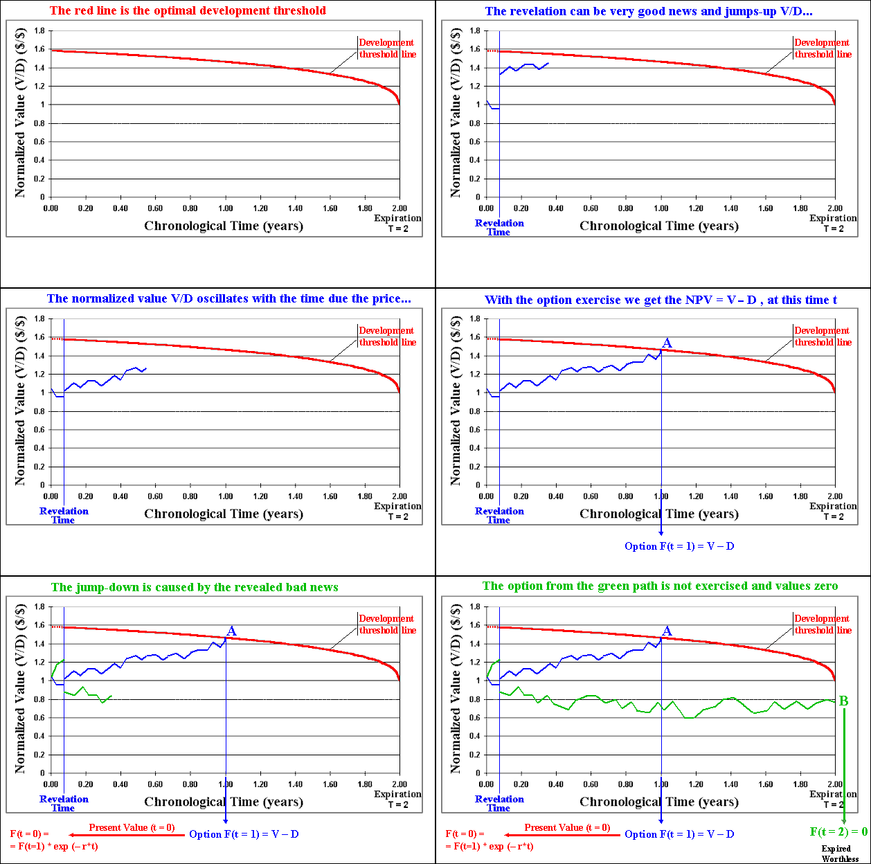
The animation above shows that the evaluation process takes the following steps:

The optimal development threshold line is traced using the efficient analytic approximation of Bjerksund & Stensland (1993), the red line in the above animation;
The investment in information takes time to learn, so that the information revelation occur in some instant between (0, 2) years;
The value of the project is function of the price of the commodity P (oil price) and, while the investment in information is performed, the normalized project value V/D oscillates due only the oil prices fluctuations. The software generates N risk-neutral sample paths of V/D;
At the moment of information revelation, almost surely the value V/D suffers a discrete-time jump because the new information changes both the producing project value V and its cost to obtain (the development cost D)
In case of good news, V/D jumps-up, and in case of bad news the value V/D jumps-down;
In each simulation sample path, the jump is the result in V and D of sampling from the revelation distributions of key parameters with technical uncertainty
After the information revelation, the value V/D continue to oscillate due the stochastic process for the commodity price (oil price), and in some cases at some instant before the expiration, the value V/D reaches or crosses the threshold line for optimal exercise of development investment ;
For the sample path with option exercise (V/D reaches the threshold) at the instant t, the option value F(t) is equal to the NPV(t) that is just the difference V - D.
However, the option needs to be evaluated at the instant t = 0. The option at t = 0, F(0) is the value F(t) time the risk-free discount factor. The use of risk-free discount rate is allowed because was used a risk-neutral simulation for the oil prices and the technical uncertainty does not demand additional risk-premium for diversified investors;
Some sample paths do not reach the optimal threshold line, and for these sample paths the option values are zero; and
After a reasonable number of simulations N, the real option value with the information is calculated as the sum of options value for all sample paths divided by the number of sample paths.

The Monte Carlo simulation is performed using a VBA (Visual Basic for Applications) software build in an Excel spreadsheet, which uses the more efficient Hybrid Quasi-Monte Carlo Approach (see the pages on Quasi-Monte Carlo Simulation for more details).

The main basic equations used in the software Timing with Dynamic Value of Information for the cases of development option exercise are:

NPV = Net Present Value = V - D

Value of Producing Project (or value of the developed reserve) = V = q P B - D.

Where q = economic quality of the reserve; P is the oil price (US$ /bbl); and B = reserve volume size.
OBS: The above equation is from the so called "Business Model". See an in depth discussion on this and others alternatives for the NPV equation in the webpage on payoff models.

D = Development Cost = Fixed Cost + Variable (with B) Cost = D_fixed + D_variable B

The above equation adjust the investment in capacity to the the reserve volume B. With the new information about the true value of B we can optimize the project using the adequate investment given by the above equation. With technical uncertainty about B, we can overinvest or underinvest in capacity losing money in both cases when compared with the case of perfect information (without technical uncertainty on B).

The variables with technical uncertainties are the reserve quality and the reserve size B. These two variables captures the key technical parameters in terms of economic relevance for the discounted cash-flow analysis, the quantity and the velocity that the reserve is sold in the market, that is, the present value of the net revenues.
The variable with market uncertainty is the oil price P, which follows a geometric Brownian motion. See why geometric Brownian motion for oil prices is not bad for real options applications (as many people think) in my online overview paper or in the Pindyck's paper in the Energy Journal, 1999.

Inputs, Outputs, Software Screens and the Registered Version

Timing with Dynamic Value of Information is an Excel applicative with VBA program that solves the problem of a real option with opportunities to invest in information, using the approach summarized here, and better described in the technical uncertainty webpage and in the paper Investment in Information in Petroleum: Real Options and Revelation.

In order to solve this problem, the software consider the following inputs:

Technical Uncertainty: the prior distributions for volume and quality of reserve;
Revelation Power from the Investment in Information: given by the expected percentage of variance reduction with the new information;
Time-to-Learn: time to gather, to process, and to interpret, transforming data into knowledge and wisdom and getting almost surely new values for the expected volume and expected quality of the reserve;
Learning Cost: the cost to invest in information, considering the whole cycle, gathering, processing, and interpretation costs;
Market Uncertainty: the oil (commodity) prices following a geometric Brownian motion (stochastic process parameters as input); and
Time-to-Expiration: the option to develop the oilfield has a legal deadline (if the development investment plan is not committed, the discovered oilfield must return to National Agengy).

The outputs from the program are:

Revelation Distributions: using the prior distributions, the revelation power inputs, and the four propositions on revelation distribution;
NPV without Technical Uncertainty: net present value based in the current expectations on the project caracteristics and market expectations;
Real Options without Technical Uncertainty: real options value based in the current expectations on the project caracteristics, market expectations, and considering the time-to-expiration;
Simulated NPV with Technical Uncertainty: consider the effect of technical uncertainty on the NPV, decreasing the NPV due to asymmetry effect of the capacity constrain;
Simulated Real Options with Technical Uncertainty but without Information Revelation: consider the effect of technical uncertainty on the real option value (ROV), decreasing the ROV due to asymmetry effect of the capacity constrain;
Simulated Real Options with Technical Uncertainty and with Information Revelation: consider that optimal investment (optimal capacity) is adjusted with the information revelation and the effect of the expected residual uncertainty (partial revelation), the optimal development option exercise after the revelation, and all the inputs.
Dynamic Net Value of Information [(6) - (5)]: The difference of the real options with and without the information revelation, net of the cost-to-learn. The term "dynamic" is because the variable time is considered: time-to-learn, time-to-expiration, and continuous-time stochastic process interacting with the techncial uncertainty.

The following pictures show the non-registered version of the software Timing with Dynamic Value of Information. The screens permit to describe some additional features of this software or to understand how to work in practice with the concepts presented before.

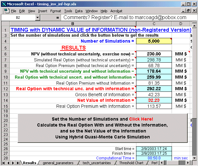
The picture below illustrates the sheet of results and also the screen to set the number of simulations (number of sample paths) and the button to start the Monte Carlo evaluation of the real options with information, the real options without information and the difference, the net value of information. The program calculates also the computational time for each simulation running. In the example below, the NPV of development is zero, but the real options value (even without information) is valuable.

The screen below is the main data input sheet. The parameters for the geometric Brownian motion for the oil prices, the expiration time, the parameter for the development cost equation, the cost of investment in information, the time to reveal the information (time to learn).

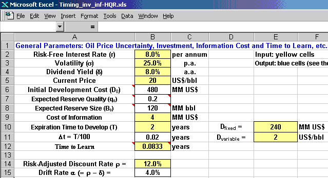
There are many inside comments into several cells, which provides a fast help for the user in a practical way. Look in the picture above the small red bullet at the upper-right corner of some cells, indicating the existence of comments.

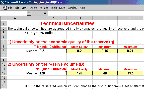
The figure below presents another sheet from the Excel file with this software. This is the screen to enter the technical parameters for the revelation distribution caused by the investment in information being considered. In the non-registered case, only the triangular distribution is available. For the registered version, there are many distributions to choose for technical parameters: Triangular, Normal, Truncated Normal, LogNormal, and Uniform.
The hybrid Quasi-Monte Carlo Simulation uses randomized Halton sequences (bases 3 and 5 for these technical uncertainties, and base 2 for the oil prices uncertainty).

In order to get an idea about the computational time, I set a screen with a table of many simulations that I performed using my personal computer Pentium III with 1 GHz of clock speed. Before setting the number of simulations, look this table in order to have an idea about the computational time (and compare your running time reported in the "results" sheet with the table below.

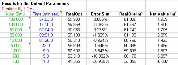
The critical threshold for the optimal development option exercise and the analytical approximation used for the real option value without information, are based in the closed-form equations from Bjerksund & Stensland ("Closed-Form Approximation of American Options", Scandinavian Journal of Management, vol.9, 1993, pp.87-99). According the Haug's textbook, this approximation is more accurate than the more popular Barone-Adesi & Whaley for long term options. This is exactly the general case of real options.

In this non-registered version, some input parameters are fixed. The fixed parameters are:

Risk-free interest rate
Dividend yield (convenience yield)
Current Oil Price
Development Time to Expiration
Variable part of the development investment

Off course in the registered version all these input parameters above are permitted to change. In addition, the technical uncertainties for both economic quality of the reserve q and the reserve volume B is not limited to the Triangular Distribution as the non-registered version. There are several distributions to choose.

Download

The link below permits the download of the non-registered version of Timing with Dynamic Value of Information, an Excel spreadsheet with facilities provided by the VBA code including a very efficient Hybrid Quasi-Monte Carlo simulator.

Download the non-registered version of Timing with Dynamic Value of Information: Compressed (.zip) Excel File timing_inv_inf-hqr.zip with 732 KB .

Alternative download: Non-compressed Excel File timing_inv_inf-hqr.xls with 796 KB .

The non-registered version is limited only by the type of probability distribution for the technical parameters (only Triangular distribution) and some few parameters are fixed (initial oil price, interest rate, dividend yield, time to expiration, and variable parameter for the development cost).

The registered version is full functional and, instead only triangular distribution for technical uncertainties, the user has 5 different distributions to choose: Triangular, Normal, Truncated Normal, LogNormal, and Uniform.
Others distributions can be added by consult (send me an e-mail).

The registered user gain the full functional version of this software and, if he/she wishes, also another version of this software using the @Risk functions (instead my VBA macro, which is faster) for the Monte Carlo simulations. With these two versions, the user can compare the results (and the computational time) of the @Risk with my version using the VBA hybrid quasi-Monte Carlo simulator.
Users of Crystal Ball that wish a registered version of Timing with Dynamic Value of Information using Crystal Ball functions, please consult me before by sending an email to marcoagd@pobox.com.

The registration fee is US$ 40, using the Gift Certificate to buy books in Amazon.com or Amazon.co.uk.
See the page about how to register software and licence fees.

Back to the Real Options Software Webpage

Back to Contents