In this webpage are presented three important concepts for evaluation and decision under uncertainty of petroleum exploration and production projects. First the concept of technical uncertainty in a modern finance framework. Second the concept of information revelation after an investment in information. The third concept is the revelation distribution (or distribution of conditional expectations), which captures the investigatory power (capacity to reduce uncertainty) of an alternative of investment in information, permitting a practical assessment to the economic value of information.
The topics presented in this webpage are:
![]() 1) Introduction and Motivation .
1) Introduction and Motivation .
![]() 2) Revelation Distribution and the Four Propositions.
2) Revelation Distribution and the Four Propositions.
. . . A Simple Numerical Example;
. . . Comparing Distributions: Prior, Posterior, and Revelation.
![]() 3) Interaction with Market Uncertainty and Timing Issues.
3) Interaction with Market Uncertainty and Timing Issues.
. . . The Best Alternative for Investment in Information and the Real Option Value.
. . . The Effect of Technical Uncertainty on the NPV function.
![]() 4) Sequential Investment in Information: Application to New Frontiers Exploration.
4) Sequential Investment in Information: Application to New Frontiers Exploration.
A) Paper: Investment in Information in Petroleum: Real Options and Revelation
B) Software: Timing with Dynamic Value of Information
![]()
The methodology presented in this webpage is applied in oilfield development projects. However, the methodology can be adapted for any project of investment in information, such as R&D (research & development), pilot projects, and market test with new products. Non-financial applications, like medical problems looking for the best treatment from a set of possible alternatives - suggested by Prof. Myers, also looks possible.
Technical uncertainty, can be solved (or revealed) with step-by-step
investment in information.
Investment in information reduces the variance of the remaining technical
uncertainty. This is very different of the economic/market uncertainty,
which uncertainty is never solved and new information is important but not
reduce the volatility of the underlying stochastic process.
In this webpage, technical uncertainty is related with the existence, the volume and the quality of an oil accumulation (oilfield reserve). The management of the revelation of the true rock/fluids properties, the technology evolution, etc., represents a great challenge for real options models that this webpage intends to contribute.
Neo-classic financial theory like CAPM (capital asset pricing model) tells that technical uncertainty has zero correlation with the market portfolio and so it does not demand risk premium by diversified investors. This is true, but it is not the whole story on technical uncertainty.
Is the risk-premium all that matters for project evaluation and decision under uncertainty? No! Managers can make more and better than just diversify technical uncertainty like shareholders. Managers can leverage value by optimal management of the technical uncertainty. In other words, managers can add significant value by optimal management of the real options created with the opportunities of (sequential or one-shot) investment in information.
In other words, CAPM remains valid but is not sufficient to perform good real world decisions about investment with relevant technical uncertainty.
The real option value is derived from the option to invest in information and, depending of the revealed information, exercise the adequate development investment option. So, there are compound options involved.
Technical uncertainty reduces the expected value of the project (the underlying asset V) because the optimal design for a project is based on the (expectation on) technical parameters (e.g., volume and quality of a reserve). If the true value for these technical parameters are different, we get a sub-optimal project, with ex-post overinvestment or underinvestment. In petroleum projects, this can be materialized by an excess or lack of wells, an excess or lack of processing capacity, etc.
In some cases, the lack of knowledge can even lead to insecurity problems in the operational phase.
The figure below illustrates the problem of sub-optimal (without information) project x optimal (with information) project, for an oilfield with technical uncertainty about the reserve volume B (number of barrels). For while imagine that the investment in information reveal the true state of the reserve volume. The decision is about the development project with a development investment D, which is function of the reserve volume, D(B), because a larger reserve requires more wells, larger capacity platform, larger diameter pipelines, etc.
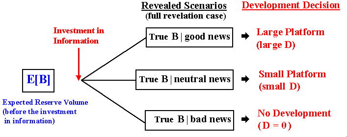
In the figure above, without complete information on the reserve volume, in order to minimize the error the project designer tends to work with the expected value (or mean) of the reserve volume E[B], by investing in a small platform. However, ex-post the decision is correct only in one scenario from three possibilities. So, in this example there is only 33% chances (if the scenarios are equally probable) of making the correct decision. There is 33% chances of underinvestment (if the true scenario is "good news" a large platform is the best alternative) and there is another 33% chances of a bad investment (in the "bad news" scenario the best is not invest due to the small reserve volume).
If we imagine that instead only three scenarios are possible dozens of scenarios or even a continuous of scenarios, the losses with suboptimal investment is even larger.
However, if the firm invest before in information, the true state of the reserve volume is revealed (for while consider perfect information or full revelation), so that the firm can make the best decision - large platform, small platform, or not investing, according the revealed scenario. This is easily quantifiable. So, optimization under uncertainty is the primary source of value of information (VOI).
In addition, with technical uncertainty we can think that the project is "deep-in-the-money" for the option exercise (development investment) when it is not. Or, we can think that the project is not deep-in-the-money, when in reality it is sufficiently profitable for the immediate development investment.
In the above example, we consider that the investment in information reveals all the truth about the reserve volume (full revelation). Typically this is a very optimistic assumption. In general the investment in information reduces the technical uncertainty but the reduction is not 100%. In most cases, investment in information gets a partial revelation of the true state of the project.
The concept of partial revelation is related with the concept of "imperfect information", whereas the concept of full revelation is related with the "perfect information" one from decision analysis literature. Lawrence (1999, p.69) states: "Perfect information occurs when the information structure provides categorical direct messages that identify precisely and unequivocally the state that occurs".
As in decision analysis literature, the value of information with partial revelation cannot exceed the value of information with full revelation (see the equivalent in decision analysis in the book of Pratt & Raiffa & Schlaifer, 1995, p.252). However, here the concept of partial revelation is introduced into a more dynamic framework, putting the revelation distributions into the real options model.
The figure below describes the example with partial revelation on the true reserve volume.
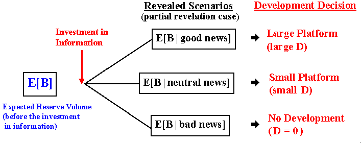
In the figure above the basic difference compared with the previous one is that, after the investment in information, the revealed scenario is described by the conditional expectation E[B | xxx news], instead "True B | xxx news" that appeared in the previous figure. This means that technical uncertainty remains in each revealed scenario - in each scenario there is a posterior distribution.
However, if the investment in information provides some relevant information (non-redundant and non-misleading information), the expected variance from the posterior distributions is lower than the variance of the prior distribution. In other words, the remaining technical uncertainty associated to the scenario E[B | xxx news] is lower than the variance associated to the prior situation associated to E[B]. This means that the problem of suboptimal decisions is less (or much less) severe with the new relevant information than without the new information. Consequently, there exists a value of information even for the partial revelation case that needs to be compared with the cost of information (the learning cost).
In the last figure, we see a set of conditional expectations scenarios after the investment in information. We can think this set as a distribution of scenarios (in the example a discrete one, but could be a continuous distribution) or a distribution of conditional expectations. I call this distribution of conditional expections of revelation distribution. This distribution is the key insight for a practical approach to capture the value of information into a dynamic framework due to its nice properties, strong theoretical basis, and easy integration with the financial concepts and models.
The paper (2002) develops a methodology to model the evolution of the technical uncertainty through four practical propositions based in the theory of conditional expectations.
Conditional expectation E[X | Y] is a random variable which takes the value E[X | Y = y] with probability P(Y = y). See the book of Sheldon Ross (1998) for a good introduction to conditional expectation without measure theory.
The concept of conditional expectation has a natural place in financial engineering computation playing a key role because the price of a derivative is simply an expectation of futures values (see Tavella's textbook, Quantitative Methods in Derivatives Pricing - An Introduction to Computational Finance, 2002, pp. vii, viii, 4).
The use of conditional expectation as basis for decisions has also strong theoretical basis. Imagine a variable with technical uncertainty X and let the new information I be a random variable defined in the same probability space (
W, S, P). We want to estimate X by observing I, using a function g( I ). The most frequent measure of quality of a predictor g(I) is its mean square error defined by MSE(g) = E[X - g( I )]2. The choice of g* that minimizes MSE(g) is exactly the conditional expectation E[X | I ]. This is a very known property used in econometrics, see for example Gallant, An Introduction to Econometric Theory - Measure Theoretic Probability with Applications to Economics 1997, pp.64-65.
Conditional expectation E[Y|X = x] is also the best regression value of Y versus X for X = x. The best regression can be linear but in general is nonlinear.
Returning to the last figure, in each scenario there is a new distribution called posterior distribution with the expected value showed in the figure. So, revelation distribution is the distribution of expectations from the posterior distributions. In this example there are only three posterior distributions, but in a more realistic setting we could think with a continuous of scenarios and, consequently, with infinite posterior distributions. Of course it is not practical to work with infinite posterior distributions. However, the revelation distribution is unique, even for infinite posterior distributions. This is a practical motivation to work with the (unique) revelation distribution, instead the (many, possibly infinite) posterior distributions.
The use of revelation distribution signifies working with all posterior distributions in a simpler and efficient way. At least, it is much less time-consuming than working with n scenarios of m posterior distributions.
The concept of revelation permits to better answer some questions:
* How to process the balance between cost and benefit of the information?
* What is the better alternative of investment in information for my
project?
This webpage intends to aswer these kind of questions. Let us start with the nice revelation distribution properties and a numerical example in the next topic.
![]()
Information revelation is the result of the investment in information,
which comprises the phases of data gathering and data processing in order
to transform information into knowledge, and knowledge into wisdom about
some key parameters in the economic evaluation of a project.
The investment in information can be costly - you spend the investment cost, or free - someone else invests in information, part of this information becomes public and you use the
information as a free-rider, see the exploratory case for the latter case.
We saw in the introduction that the revelation distribution represents the possible scenarios for the
expected value of a parameter after the information revelation. Revelation distribution is the conditional expectations distribution, where the conditioning is the new information revealed by the investment in information.
Revelation is a process towards the truth. Here this denomination emphasizes the change of expectations with the revealed new scenario and the learning process or discovery process towards the true value of the variable.
This revelation concept has similarities and differences with the famous principle of revelation, from the literature of asymmetric information (or more specifically the theory of mechanism design) and in Bayesian games in general. Our setting means the revelation of the true value of the technical parameter (true state of the nature of one parameter), whereas the mechanism design concept is related with the true type of one agent (a direct mechanism designed to be optimal for a player to say the truth).
Definition: Let X be the variable with technical uncertainty (e.g., the reserve volume B), and the investment in information reveals the information I = i. Revelation distribution is defined as the distribution of RX = E[X | I]. The revelation distribution properties such us the mean and variance, are presented below as propositions.
The highest efficiency for one investment in information is when it reduces to zero the variance of the posterior distribution, resulting in a full revelation (reveal the truth on the technical parameter). Recall the first figure presented at introduction.
What are the possible scenarios after this very efficient investment in information? Of course, ex-ante all the scenarios from the previous total uncertainty (prior distribution) are possible. If not, our prior distribution is not representative of the (total) technical uncertainty in the project. Hence, in case of full revelation, the revelation distribution must be simply equal to the prior distribution, and it is the first proposition. The analysis is by ex-ante perspective because we need to decide to invest or not in additional information. Of course that ex-post we can discover that we underestimate the technical uncertainty, but here we consider that the project team makes ex-ante reasonable and non-biased estimates about the project uncertainties - if not, "garbage in, garbage out", it is not a modeling problem.
We also saw in the introduction that is much more common the case of partial revelation, that is, the investment in information reduces the uncertainty but not completely. In this case the revelation distribution is not equal to the prior distribution, so that we need to characterize the revelation distribution for the partial revelation cases. What is the mean of this revelation distribution. What is the variance? How evolve the revelation distributions in a sequential investment in information setting? The answer to these three questions are the propositions 2, 3 and 4, respectively.
Let us see the four propostions, which characterizes the process of learning for technical uncertainty.
The Four Propositions for the Revelation Distribution:
The first proposition is trivial - but very important as the limiting of a learning process, and it draws directly from the definition of prior distribution. The others three propositions are demonstrated in the paper appendixes
The second proposition is just an application of the law of iterated expectations. The third proposition is the central proposition because captures the revelation power of one investment in information, that is, the capacity of a learning process to reduce the uncertainty, which is directly linked to the revelation distribution variance. The last proposition helps the evaluation of different plans of sequential investment in information, permitting the application of martingale tools that is a well developed branch in probability and stochastic processes.
With the reasonable assumption that the prior distribution has finite mean and variance, Proposition 1 tells that even with infinite quantity of information, the variance of revelation distribution is bounded. This contrasts strongly with some real options papers that model technical uncertainty using Brownian motion, which the variance is unbounded and grows with the simple passage of time, which is also inadequate - this distribution changes only with new relevant information is revealed through investment in information.
About the last point, the figure below illustrates the difference of a continuous-time stochastic process (from a market variable like the oil price) and the evolution of a technical uncertainty (e.g., the reserve volume B). The figure shows one typical sample-path in each case along the time. The market variable changes with the simple passage of the time because every day investors expectations on the supply and demand are tested in the market, whereas the expected volume of a reserve changes only if new relevant information arrives from a new investment in information (in some cases due to new technology, but this is even more dispersed in discrete points along the time).
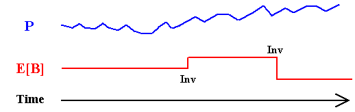
Hence, the technical uncertainty evolves in discrete-time fashion and in most cases is an event-driven process controled by the manager. That is, the manager has the option to invest in information and, if it is exercised, almost surely will obtain a new expectation for the technical parameter(s).
The above propositions allow a practical way to ask the technical expert in order to get the information necessary to model technical uncertainty in this approach. Only two questions:
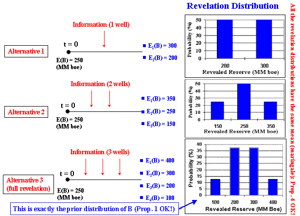
Let us see a simple numerical example in order to illustrate the propositions, to see the differences between posterior distributions and revelation distribution, and to develop the intuition about the sequential investment in information.
This simple example illustrates the concept of revelation distribution for a technical parameter value - the reserve volume B of one oilfield. Recall that this distribution is just the probability mapping of the possible expected values for this parameter after the information revelation.
The example below is stylized in the sense that is a very simplified version
from the oilfield reality. However, due to the example simplicity the
main idea (concept of revelation distribution) is more clearly explained.
Suppose the following stylized delineation of an oilfield (appraisal phase of a discovered oilfield). The drilled well in the area "a" proved 100 million boe (boe = barrels of equivalent oil, that considers oil + gas). However, there are technical uncertainty about the volume of the others three areas (b, c, and d).
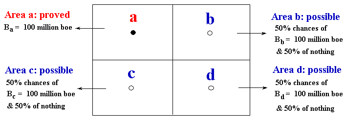
In this example, each well reveal all the truth in its respective area. For example, the appraisal well in the area "b" will say all the truth if that specific area has more one hundred million barrels or zero. The others appraisal wells cases are analogous - as showed in the figure above.
The Alternatives of Investment in Information: This investment in information is an option, not an obligation. So the alternative zero is not invest in information (we can develop the oilfield or not without additional information).
Assume that there are three mutually exclusive alternatives of investments in information, besides the alternative zero of not investing in information.
The alternative 1 drills one appraisal well in the area "b" and revel all about that area, but nothing about the remaining areas "c" and "d" (partial revelation). The alternative 2 have a higher revelation power because drills two appraisal wells (e.g., in the areas "b" and "c"). The alternative 3 have the highest power revelation by drilling three appraisal wells, and in this example this means the condition of full revelation.
Initially, let us consider that all alternatives are
one-shot investment. That is, initially forget the sequential investment in
information process for the alternatives 2 and 3.
The idea here is to show that alternatives with more revelation power
(more power to reduce the technical uncertainty) has a revelation
distribution with higher variance. Let us to detail the alternatives
in the following slides.
First note that the initial uncertainty (unconditional distribution) also known as the prior distribution, is represented by the following discrete scenarios distribution:
Hence, the expected value for the unconditional distribution is E[B] = 250 million bbl and the variance is Var[B] = 7500 (million bbl)2.
Let us see what happen with the different investments in information, in both the posterior (or conditional) distributions and the revelation distribution.
The revelation distribution obtained with one alternative is the distribution of expectations after the information revelation for this alternative. What are the new possible scenarios of expectation after the appraisal drilling in the area b (Alternative 1)?
Alternative 1 generate two possible scenarios, because the well b result can be success proving more 100 million bbl (positive revelation with 50% chances) or dry (negative revelation with 50% chances). These two scenarios of new expectations revealed with one appraisal well, form the discrete revelation distribution for Alternative 1. This revelation distribution is a discrete distribution with two scenarios, which are presented below.
Note that, with the Alternative 1, it is impossible to reach more extreme scenarios of revelation such us 100 million bbl or 400 million bbl. This is because the revelation power of Alternative 1 is not sufficient to change the expectation of the entire reserve so much to reach extreme cases.
Alternative 1 reaches only a partial revelation, so that the uncertainty remains and the posterior distribution B|A1 has variance nonzero. What is the expected variance for the posterior distributions with the Alternative 1?
In case of positive revelation, the posterior distribution is {200 million bbl with 25 % chances; 300 million bbl with 50 % chances; and 400 million bbl with 25 % chances}. For the negative revelation scenario, the other posterior distribution is {100 million bbl with 25% chances; 200 million bbl with 50% chances; and 300 million bbl with 25% chances}.
The reader can calculate that the remaining variance (variance of posterior distribution) in both scenarios of revelation are 5000 (million bbl)2, and so the expected variance of posterior distribution is also 5000 (million bbl)2. So, Alternative 1 reduces the variance of B in 33% (from 7500 to 5000). In this simple example, this is also the searched area in relation to the total area with uncertainty.
Let us check the Propositions 2 and 3. The expected value of the revelation distribution for the Alternative 1 is:
EA1[RB] = 50% x E(B|A1 = good news) + 50% x E(B|A1 = bad news) = 250 million bbl
As expected by the Proposition 2!
The variance of the revelation distribution for Alternative 1 is:
VarA1[RB] = 50% x (300 - 250)2 + 50% x (200 - 250)2 = 2500 (million bbl)2
As expected by the Proposition 3, the variance of revelation distribution is equal to the expected reduction of variance caused by the investment in information (7500 - 5000)!
The reader can check the Propositions 2 and 3 for the Alternatives 2 and 3, and the Proposition 1 for Alternative 3 (full revelation). The reduction of variance of Alternative 2 is 66% (from 7500 to 2500), whereas the reduction of variance for Alternative 3 is 100% (from 7500 to zero).
The figure below shows the revelation distributions for the three alternatives. Note that, as higher is the revelation power as higher is the variance of revelation distribution. Note also that the revelation distribution for the Alternative 3 (full revelation) is exactly the prior distribution, as required by Proposition 1. In addition, the figure shows that all alternatives the means from the revelation distributions are equal to the original (prior) expected value (250 million bbl).
What is the class (shape) of the revelation distribution in case of partial revelation? In general it depends of the distribution of the outcomes from the new set of information (e.g., for Alternative 1, a discrete distribution with 50% success and 50% for dry well). More precisely (see Goldberger, 1991, p.49), it depends on the joint probability density function (joint pdf) of reserve B with Alternative 1.
For the limiting case (full revelation), Proposition 1 tells that revelation distribution and the prior distribution are of the same class (in reality are equal). Even the partial revelation distributions having different shapes (look the previous figure to see this), as the variance grows the shapes of these distributions evolve towards the prior distribution shape. For practical simplicity assume that the revelation distribution class is the same of the prior distribution of technical parameter. This is absolutely correct for the full revelation case and a practical simplification for the partial revelation case. If the variances (given by the Proposition 3) are the same, differences in the distribution shapes generally have secondary numerical effects on the real option value. Hence, if we use a triangular distribution for the prior distribution, the revelation distributions will be triangular too.
The (Bayesian) prior (or a priori) distribution
is the estimated initial uncertainty without any learning (before invest in
information). Recall the beginning of the numerical example.
It can be a subjective evaluation of uncertainty, but for the case of appraisal phase of a discovered non-developed oilfield there are previously cumulated information (knowledge) of the oilfield, so that the objective information plus a some degree of subjective interpretation. The description of the current (residual) uncertainty is the prior distribution, in this probabilistic and quantitative setting.
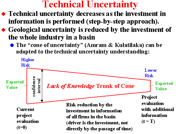
The Bayesian's posterior (or a posteriori) distribution is the prior distribution updated with the new information, for each possible new information outcome. Learning means that the mean variance of the posterior distributions is lower than the variance of the prior distribution, reflecting the reduction of the uncertainty of the parameter (see the inverted cone of uncertainty in the example on exploration of basins).
The revelation distribution variance is related with the investigatory
power of an investment in information. As higher is the investigatory
power, as higher is the revelation distribution variance.
So, when the variance of posterior distributions decrease, the revelation distribution variance increases. Learning has opposite effects in these variances.
As the variance of the revelation distribution is inversely related to
the variance of the (Bayesian's) a posteriori distribution, is natural
that Bayesian methods can be used to find the revelation distribution.
However, some rules of consistency are necessary and I advocate that these rules shall be four propositions presented. For example, an alternative of investment in information that reveal all the truth about
one parameter (the alternative 3 in the example above), that is, the full
revelation alternative, has a revelation distribution equal to the
Bayesian's prior distribution (proposition 1). Full investigatory power means that the
alternative investigates all the possibilities described by the prior distribution.
I think that this case limit is important to understand better the concept of revelation distribution. For alternatives with inferior
investigatory power, seems natural to think that the revelation
distribution has lower variance (lower explanatory power) than the
Bayesian's a priori distribution.
The picture below, illustrates the four propositions and compares one of the possible posterior distributions with the unique revelation distribution:
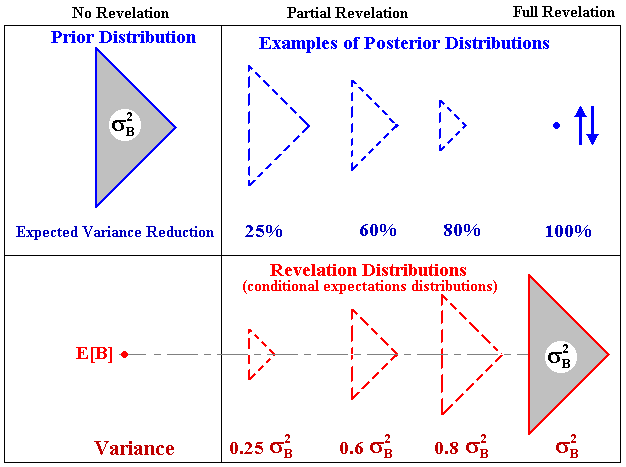
Note in the picture above that the variance of revelation distribution is equal to the expected variance reduction (proposition 3).
This picture helps to answer the apparent paradox: if the real options value is increasing function of volatility, what is the advantage to reduce the technical uncertainty? Or as asked by Martzoukos & Trigeorgis (2001), why learn? The answer is that in economic analysis of projects (and in finance in general) we work with (conditional) expectations, that is, with the revelation distribution, and not with one particular posterior distribution. As large is the expected reduction of the technical uncertainty as large is the variance of the revelation distribution and hence the real options value.
So, learning increases the real option value! With the revelation distribution is easy to see why.
Sequential Investment in Information
Imagine you are searching the optimal sequential investment in information plan. One alternative with a great investigatory power for the first investment in information means expected low variance for the posterior distributions. However, this reduces the incentive to set a second investment in information in this appraisal plan, because the variance of revelation distribution with the second investment is limited by the (low) expected variance of the first set of posterior distributions.
Returning to our stylized example of rectangular oilfield, consider the case of two sequential investment in information (alternative 2). See the posterior distributions (in green, 3 distributions with two scenarios each) after the two sequential investments, and the unique revelation distribution (in blue, with three scenarios) .
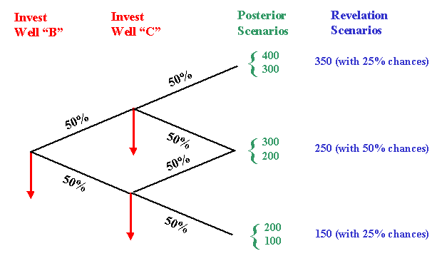
Note that the revelation distribution after two sequential investments is a martingale (the mean is 250 as before), consistent with the proposition 4.
In practice, searching plans with two sequential investment require that
the possible revealed scenarios from the first appraisal investment have
low redundancy with the revealed scenarios from the second appraisal
investment. For example, in the appraisal phase of an oilfield the
sequential drilled wells are placed relatively far from the other, in
order to check out the oil existence and quality in different points of
the a priori mapped probable/possible area.
In the simple numerical example, the information was always non-redundant and independent (no correlation between the wells).
In real life can occur some degree of redundancy and/or correlation. The four propositions presented above remains true even in these cases. However, some experience and perhaps some additional probabilistic analysis can be necessary to estimate the key insight that is the expected reduction of variance (the expected learning) with a specific project of investment in information.
From a managerial point of view, expected reduction of uncertainty is a sound concept to work when analyzing projects of investment in information. The use of this concept in corporations will help the communication inside the organization to analyze these kind of project and to compare the alternatives of learning.
![]()
How is the relation between technical variables - like volume and quality of a reserve, and market variables like oil prices in the net present value (NPV) function?
Assume that we have discounted cash flow spreadsheet, with an estimate of the NPV using an oil price P. Assume we can use a linear model for NPV(P) = V(P) - D. Consider the Business Model for the oilfield development project. The chart NPV versus P for this model is showed in the figure below.
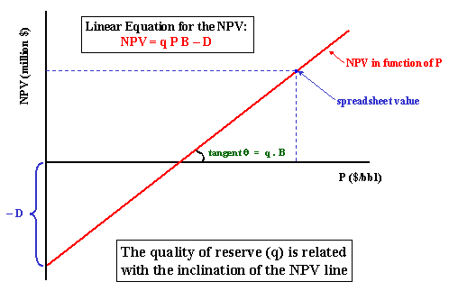
Note that the inclination is the product q B.
For details about this and others NPV(P) linear (and also for non-linear) models, see the webpage Linear and Nonlinear Models for the Underlying Asset V(P) and the NPV Equation
The net present value equation for the oilfield development in this model is function of the (expected) volume of reserve of B, the (expected) quality of reserve q, and the development investment D (in present value and net of fiscal benefits). The market uncertainty is represented by the (long run current expectation on) oil price P that follows a geometric Brownian motion.
NPV = q P B - D
Assume that the optimal capacity is function only of the reserve volume B, and this optimal development investment is a linear function D(B) given by:
D = FC + VC . B
Where FC is a kind of fixed cost (minimal investment to produce anything) and VC is a variable cost parameter.
This equation is used after a revelation for the optimal capacity choice given the new information about B.
See also the effect of technical uncertainty on the NPV function, with additional considerations for the loss of value in the NPV equation due to the remaining technical uncertainty.
The figure below illustrates the combination of technical uncertainty (one-shot revelation distribution) with continuous-time market uncertainty (stochastic process for the oil prices), and considering the time-to-learn, the time to expiration of the option to develop the oilfield.
The figure presents two sample paths from the Monte Carlo simulation. This approach combines continuous-time risk-neutral geometric Brownian simulation of oil prices with the simulation of the revelation distributions from the technical uncertainties. This combination occurs at the "revelation time", when almost sure we have changes in the expectations on both the reserve size and the reserve quality (hence in V/D).
It also shows the normalized threshold curve (V/D)* that is the same for any revealed scenario! See the paper for details.
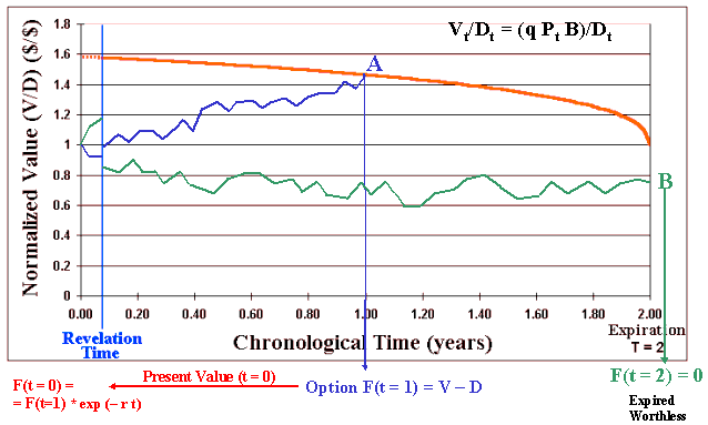
It also considers two years for the expiration of the development rights and shows how the simulated sample paths are evaluated in this real options model.
In the general model, the development cost D could have a multiplicative market uncertainty component following a correlated geometric Brownian motion. The normalized threshold curve remains valid even in this case for the optimal exercise of the option to develop.
In the first sample path (blue) showed in the above figure, the normalized value V/D evolves randomly due the risk-neutral simulation of the oil prices component. At the revelation time are drawn one sample from each revelation distribution (q and B) and the normalized value of reserve jumps (in this case jumps-up) almost surely, reflecting the new expectation on these technical parameters in this path. The value V/D continues its random trajectory, now due the (long-run expectation) oil price oscillations. In this path V/D reaches the threshold curve at the point A (see the picture). The option is optimally exercised and multiplied by the risk-free discount rate factor, in order to calculate the present value.
The risk-free discount rate is used because the technical uncertainty doesn't demand risk-premium for diversified shareholders (no correlation with the market portfolio) and the market uncertainty is already penalized with the risk-neutral measure.
The second sample path (green) evolves similarly but after suffering a jump-down from the samples of revelation distributions, the path evolves until the expiration without reaching the threshold line and expires worthless (point B). The option value F for this path i is zero, and negative for Wi, where Wi is the real option value net of the cost of information.
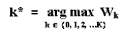
After thousands of simulated paths, we get an estimative of the real options value by summing up the options value Fi of all sample paths and dividing by the number of simulations (sample paths). Subtracting the cost to learn Ck we find the real option value Wk for the alternative k. Repeat the process for each one of the k alternatives and select the best alternative k*, the alternative with the higher Wk.
This is exactly the procedure used by the software Timing with Dynamic Value of Information.
Now, imagine that the firm didn't invest in information. What happens with the green sample-path? Look the figure and imagine a parallel green sample-path so that there is no jump at the revelation-time. It is easy to imagine that this sample-path could reach the threshold curve a little bit time before the expiration so that the firm could invest in this case. However, with information, we see that the (true or almost true) expected NPV is negative for this path. Let us put numbers. If the investment is US$ 1 billion, the NPV is in reality worse than US$ 200 millions. So, the informed manager could prevent losses of US$ 200 millions in this example by investing in information before. Investment in information in petroleum - like one additional appraisal well, could cost only US$ 10 million - a small fraction of the development investment.
See also in the "Timing with Dynamic Value of Information" webpage, an animation and additional explanation about the methodology summarized above.
Consider that there are K alternatives of investment in information, k = 0, 1, 2, �K (being k = 0 is the alternative of not investing in information). Assume for the alternative k that the cost of learning is Ck and the time to learn is tk. So, the model considers that learning takes time, penalizing the alternatives that demands much time to reveal the information/knowledge. Initially imagine that the investment in information starts always at the initial instant (t = 0), see section 6.1 a discussion on timing of learning. Let Wk be the value of the real option including the cost and benefit of the alternative k. The aim is to choose the alternative k* with the highest Wk. Formally:
The value Wk is the value of the (American) real option to develop the oilfield after (or conditional to) the partial revelation of the technical uncertainty with the alternative k, net of the learning cost Ck. That is, it is the benefit less the cost of the information, given by the following equation :
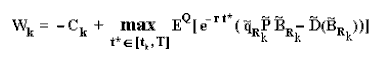
Where EQ is the expectation under risk-neutral (martingale) measure, permitting to calculate the expected present value of the payoff (NPV for development) using the risk-free discount rate. The expectation is also conditional to the information revealed by alternative k (but not charged in the notation). This expectation is calculated using a Monte Carlo simulation. The tilde represents stochastic variables, being P(t) and possibly D(t) following risk-neutral GBMs, and the technical variables (with subscripts Rk) drawn from the revelation distributions (or conditional expectations functions) generated specifically by the alternative k, at the instant tk.
The value Wk is maximized by optimal timing choice of the option exercise t* (called stopping time by the mathematicians) in the interval from the revelation time of alternative k, tk, until the expiration T. In the Monte Carlo simulation, the stopping time for the sample path i is the first time that the normalized value of the project V/D reaches the normalized threshold (V/D)*. Formally:
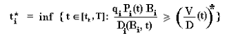
With the standard convention that the infimum of an empty set is + infinite, so that for the empty set (for a path without exercise) the value inside EQ(.) in the equation Wk, is zero.
I invite the reader to return back the chart with the sample-paths and threshold curve, and compare the logic of these two last equations with the visual approach presented in the chart.
The net present value equation NPV = V - D = q P B - D(B) is based on the expected value for the cash-flows, and it is necessary answer the following question:
Is the NPV the same if we have no technical uncertainty on q and B compared with the case with technical uncertainty and using E[q] and E[B]?
The answer is negative and both the reason and how to proceed are given below.
The theory of finance tells that technical uncertainty (like the uncertainty on reserve volume B), being independent of the market portfolio, it doesn't demand risk-premium because the stockholders of the firm are diversified investors.
However, the optimal management of technical uncertainty is appreciated by the investors because can leverage value either by optimal management of the opportunities of investment in information, as by the more valuable exercise of option to develop the oilfield using an optimized alternative of development.
The exercise of the option to develop without knowing the correct reserve volume B and the technical factors affecting the quality of the reserve, almost surely will conduct to a sub-optimal development (e.g., see the cases reported in Demirmen, 2001). Let us quantify the losses with sub-optimal development.
Instead a risk-aversion on technical uncertainty, is used a loss factor penalizing V due to the probability of sub-optimal development. In short, from moderm finance theory point of view, technical uncertainty it is not a matter of choice of an utility function to express the risk-aversion. The problem with technical uncertainty is that it reduces the firm value due the lack of optimization projects, e.g., by investing more than the necessary or less than the optimal level.
With a better information on the reserve volume B we can fit better the investment D to its volume B. It was partially performed in this model because the investment cost D is a function of the reserve B and because is considered the optional nature of development. For example, knowing that B is lower than expected, we can reduce D. Without this information, using a higher investment D than the necessary it is possible to exercise options with apparent positive NPV in some scenarios of B, which could be ex-post negative due to the revealed lower reserve volume B.
Let us recall the NPV equation for the oilfield development (using the "Business Model") as function of the oil price (P), the economic quality of the developed reserve (q), the reserve volume (B), and the development investment (D):
NPV = q P B - D
Recall that the quality q is related with the present value of net revenues, that is, with the speed that the reserves are extracted and sold in the market.
If the capital in place is sub-dimensioned for the reserve volume (revealed B is higher than expected), then the capacity constrains reduce the associated value of q. This occurs because even if all the reserve volume B can be extracted with the sub-dimensioned capital D, the present value of reserve (the product q P B) is lower due the slower extraction rate. This limitation suggests a penalty factor for the quality q for the cases where the reserve volume reveals higher than expected.
The same reasoning is possible if the average well productivity is higher than expected. Let us call this penalty factor of γup, which is defined in the interval (0, 1]. This factor penalizes the value of the developed reserve V if the ex-post q B > E[q B].
This penalty factor is not derived from "risk aversion of managers on technical uncertainty" or "manager's utility" as used in traditional decision analysis literature. The penalty factors will be derived from discounted cash flow analysis of value lost due the reserves production with limited capacity system and sub-optimal location for the wells. The method presented in this paper is simple, but more sophisticated methods can be used for the penalty factors.
We could define another penalty factor γdown for the cases where the capital in place D reveals over-dimensioned for the reserve size and/or for the average well productivity. However, some empirical studies have been showing this value is near one. In this case, even without penalizing V, recall that the project NPV is already penalized because D is higher than the necessary.
In general, the NPV function with remaining technical uncertainties can be estimate with a Monte Carlo simulation of the distributions of q and B, by using the following equations (for practical cases, we can make γdown = 1):
To apply these equations, the remaining issue is how to estimate the value of the penalty factors. It can be done using discounted cash flow analysis by fixing the investment (capacity) and calculating the present value of the net revenues (that is, calculating V) for different scenarios for q and B.
A practical way to estimate γ is by performing this analysis for a few representative scenarios of the technical distribution and assuming that the penalty factors changes only with the variance of the technical uncertainty. For the partial revelation case (even with new information there is a remaining technical uncertainty) the penalty factor must be updated to a value between the previous value of γ (without information) and the penalty factor for the full revelation case (for the full revelation, γ = 1). If we build some rule of update for γ such us "the difference between g and 1 is proportional to the remaining variance of technical uncertainty", it is easy to update the value of γ without the necessity of running additional DCF analysis for different levels of partial revelation. With this rule, for the case of zero variance for technical uncertainty the factor γ is equal to one (not penalizing the NPV).
By using the practical updating procedure above for γ, we need only to estimate the penalty factors for the initial technical uncertainty (before the investment in information). One suggestion is to reduce the technical uncertainty distribution into three scenarios: upside, expected, and downside. By running the DCF analysis for these scenarios with and without full information, with D projected for the expected case, we have typically the values of V displayed in the figure below.
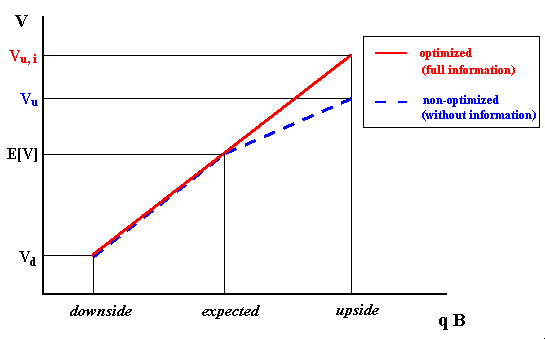
The picture above illustrates a case with γdown = 1 (the value Vd is the same for the cases with and without information, but not the NPV due the effect of D). The penalty factor γup and the non-optimized value are given simply by:
The reserve value without full information is an intermediate value between the expected reserve value and the reserve value with full information.
In this way, a Monte Carlo simulation is performed using the above equations in order to see that, under technical uncertainty, the value E[V] is lower than E[q P B] if D is fixed.
To update the factor γ and so the NPV after a partial revelation, is possible to perform many simulations with capacity constrains for different levels of variance for the technical uncertainty. However, in our examples is used a simpler framework. This factor tends to 1 when the variance of the technical uncertainty is equal zero. So, we can think in this equation for the updating with the process of reduction of variance, where bi = before information and ai = after information:
γai = γbi + (1 - γbi ) [% variance reduction(B) + % variance reduction(q)] / 2
In short, this section showed a methodology to consider the loss in value due the lack of information (technical uncertainty). The value of information is related with the optimal choice of capacity. This affects both the optimal investment D and the present value of net revenue (V). The former is considered through the equation relating D with the reserve volume B, whereas the latter is considered by the penalty factor γ.
![]()
This topic illustrates the general case of revelation for a sequential investment in information process. The example is a relatively little explored basin with uncertain oil and gas potential.
An oil company can acquire tracts in that basin with substantial technical uncertainty. In other words, oil companies acquire investment options. With the passage of the time, the firms acting in that basin will invest in exploration and will reveal new information about the basin potential. The new information is partially revealed to the public - firms have to inform stock markets and national agencies about relevant news about exploratory investment.
Even in the exploratory case with many "players" (firms), the arrival of new information is not continuous: a new relevant information can take months - or even years in some cases, to arrive. So that the use of continuous-time stochastic process like the geometric Brownian motion remains being a misunderstanding. However, the modeling of information arrival with a Poisson process - perhaps non-homogeneous Poisson process due to the "cascade effect" with good news, can be a good alternative for this modeling.
The time to expiration of the rights for these exploratory tracts generally ranges from 5 to 10 years, so that there are good chances to use new information for investment decisions due to both itself exploratory investment and exploratory investment from others companies. In the last case, the firm that uses the information generated by the other firms is named "free-rider", because the firm gets information without cost.
The slides below illustrate this exploratory problem in little explorated basins.
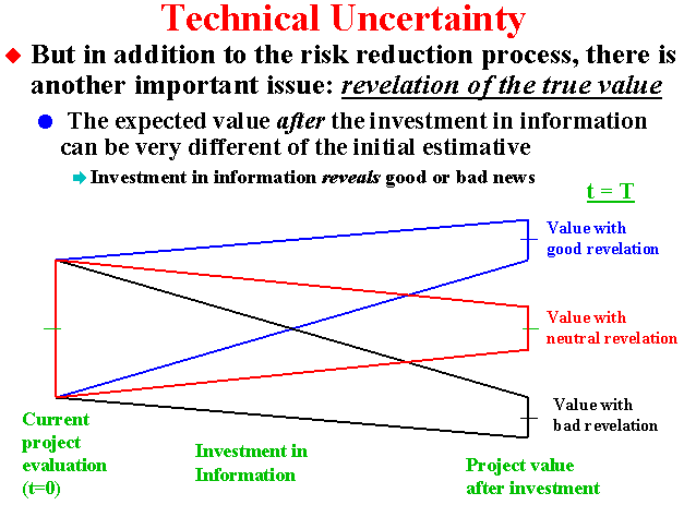
In addition to the variance reduction, even more important is the revelation of the true value.
Information can be costly (our investment) and/or free, from the other firms investment (free-rider).

![]()
This paper was presented first at the MIT Seminar "Real Options in Real Life", May 2nd, 2002.
After that, I have been presenting it in many conferences: "6th Annual International Conference on Real Options", Cyprus, July 2002; the "SPE Applied Technology Workshop", Rio de Janeiro, August 2002; and in the "Workshop on Real Options and Energy", Mexico City, September 2002.
See the webpage Real Options Online Multimedia Material for Powerpoint files and other materials related to these seminars/workshops/conferences.
The paper presents the main issues presented in this webpage, including the four propositions
to characterize the technical uncertainty and the learning process through
the concept of revelation distribution. In this paper I set for the first time these nice properties of the revelation distribution, although I have been working with the concept of revelation distribution since 1997/8.
Download the paper using one of the links below:
![]() Download the Word for Windows file
marco_dias_revelation.doc, with 988 KB.
Download the Word for Windows file
marco_dias_revelation.doc, with 988 KB.
Or download the compressed (.zip) version:
![]() Download the Compressed (.zip) Word for Windows file
marco_dias_revelation.zip, with 156 KB.
Download the Compressed (.zip) Word for Windows file
marco_dias_revelation.zip, with 156 KB.
Next I present the paper abstract from the last version (December 2002).
Abstract
A firm owns the investment rights over one undeveloped oilfield with technical uncertainties on the size and quality of the reserve. In addition, the long run expected oil price follows a stochastic process. Expectations drive the valuation of the development option exercise. The modeling of technical uncertainty uses the practical concept of revelation distribution, the distribution of conditional expectations where the conditioning is the information revealed by the investment in information. The paper presents 4 propositions that helps the firm to select the best alternative of investment in information with different learning costs and different benefits in terms of capacity to reduce uncertainty. This technical uncertainty modeling is practical because is necessary to know only the initial uncertainty (prior distribution) and the revelation power, defined as the expected percentage of variance reduction induced by the alternative of investment in information. The model includes a penalty factor for the lack of information, which causes sub-optimal development, and this factor is introduced into the dynamic real options model. After the information revelation, the optimal development decision depends on the project value normalized by the development cost. This normalized threshold is the same for any technical scenario revealed by the new information when the oil price follows a geometric Brownian motion. In addition, there is a time to expiration of the rights for the option to develop. The model outputs are the real options value with and without the technical uncertainty, with and without the information, and the dynamic value of information.
Keywords: real options, investment under uncertainty, investment in information, value of information, learning options, valuation of learning projects, conditional expectations approach, technical uncertainty, information revelation, revelation distribution.
![]()
Timing with Dynamic Value of Information is an Excel applicative with VBA program that solves the problem of a real option with opportunities to invest in information, using the approach described in this webpage and in the paper Investment in Information in Petroleum, Real Options and Revelation.
In order to solve this problem, the software consider the following inputs:
The outputs from the program are:
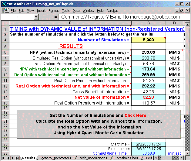
The figure below presents the sheet with the main outputs of this software.
More details on this software, see the webpage Timing with Dynamic Value of Information, with animation illustrating the interaction of technical uncertainty with market uncertainty in the evaluation process, others screens, additional discussion on software features, etc.
The link below permits the download of the non-registered version of Timing with Dynamic Value of Information, an Excel spreadsheet with facilities provided by the VBA code including a very efficient Hybrid Quasi-Monte Carlo simulator.
![]() Download
the non-registered version of Timing with Dynamic Value of Information:
Compressed (.zip) Excel File timing_inv_inf-hqr.zip
with 732 KB.
Download
the non-registered version of Timing with Dynamic Value of Information:
Compressed (.zip) Excel File timing_inv_inf-hqr.zip
with 732 KB.
![]() Alternative
download: Non-compressed Excel File timing_inv_inf-hqr.xls
with 796 KB.
Alternative
download: Non-compressed Excel File timing_inv_inf-hqr.xls
with 796 KB.
The non-registered version is limited only by the type of probability distribution for the technical parameters (only Triangular distribution) and some few parameters are fixed (initial oil price, interest rate, dividend yield, time to expiration, and variable parameter for the development cost).
The registered version is full functional and, instead only
triangular distribution for technical uncertainties, the user has 5
different distributions to choose: Triangular, Normal, Truncated Normal,
LogNormal, and Uniform.
Others distributions can be added by consult (send me an e-mail).
This paper is an application of evolutionary real options approach for the evaluation and selection of the best alternative of investment in information, before an oilfield development. Evolutionary Real Options approach is a kind of hybrid real option which combines the real options approach with techniques of evolutionary computation, such as genetic algorithms. The abstract is placed after the download links.
The file below is the Powerpoint presentation of my speech at the "5th
Annual International Conference on Real Options - Theory Meets Practice",
UCLA, Los Angeles, July 13-14, 2001.
The title of the this presentation is "Selection of Alternatives of
Investment in Information for Oilfield Development Using Evolutionary Real
Options Approach".
![]() Download the Powerpoint 97 file: inform-evol_ro-dias.ppt,
with 953 KB
Download the Powerpoint 97 file: inform-evol_ro-dias.ppt,
with 953 KB
Use the full screen (or presentation mode) in the Powerpoint, in order
to see the animation. The file above was save without the embedding
true-type fonts (which enlarge a lot the size).
If you don't have the fonts or experimented any problem with the fonts,
you can download the compressed Powerpoint file with embedded true-type
fonts below:
![]() Download the compressed Powerpoint 97 file with embedded true-type
fonts: inform-evol_ro-dias-true_type.zip,
with 2,027 KB.
Download the compressed Powerpoint 97 file with embedded true-type
fonts: inform-evol_ro-dias-true_type.zip,
with 2,027 KB.
The paper correspondent to this presentation is also available to download (compressed Word file):
![]() Download the paper in compressed Word 97 for Windows:
evol_ro-marco_dias.zip, with 594 KB.
Download the paper in compressed Word 97 for Windows:
evol_ro-marco_dias.zip, with 594 KB.
Abstract
Consider an undeveloped oilfield with uncertainty about the size and quality of its reserves. There are some alternatives to invest in information to reduce the risk and to reveal some characteristics of the reserve. This paper presents an evolutionary real options model of optimization under uncertainty with genetic algorithms and Monte Carlo simulation, to select the best alternative of investment in information. There is a legal time to expiration of the option to start the investment for the oilfield development. The model considers both the technical uncertainties revealed by the information and the market uncertainty using two different stochastic processes for the oil prices, which are simulated. Monte Carlo simulations evaluate the decision rule curves generated in the evolutionary process. The process evolves toward a near optimum solution, giving the real option value and the optimal decision rule. The evolutionary programming under uncertainty was performed in C++ environment with good results and a description of the programming procedure is provided.
Back to Timing with Dynamic Value of Information