Most applicative cases in the Real Options Software Section are spreadsheet applications in Excel using Visual Basic for Applications - VBA - with macros and user defined functions. Let us see the list:
The three components of the Timing Suite are the Timing
basic; Timing with two stochastic variables (project value and
development cost); and Timing for the option to switch use (also
with two stochastic variables, but here analogous to a put instead a
call).
The only available shareware to download is Timing in its basic version.
The others are described below. Interested people to acquire a licence of
these software, click here.
All these modules of the Timing Suite in Excel format calculate:
There are two charts which are updated automatically when you change
the value from the parameters:
Option value chart and threshold chart (the free-boundary)
that gives the optimal decision rule.
Using spinners to change the parameters, you can see (like an Excel "movie")
the lines in the charts moving.
I divided the Excel window into two panels: in the upper panel is
displayed the data input entry and in the lower panel the solutions mainly
for option value and threshold, including charts.
The new Timing version has many important differences compared with the older Timing version:
First, now it is using VBA (Visual Basic for Applications) macros
and user-defined functions. By using VBA, the spreadsheet size is
lower and faster than the previous Timing version. In addition, it permits
to perform a Monte Carlo simulation by using macros.
The VBA code is password protected, but the references given here permit
the interested reader to access the sources (formulas and algorithm codes
in some cases) and build a code by him/herself, or even to check the
results obtained with Timing.
Second, this version uses a better analytical approximation due to
Bjerksund & Stensland ("Closed-Form Approximation of American
Options", Scandinavian Journal of Management, vol.9, 1993,
pp.87-99), replacing the popular Barone-Adesi & Whaley's analytical
approximation used in the previous version of the Timing Suite.
According the Haug's book (The Complete Guide to Option Pricing
Formulas, McGraw-Hill, 1998), which this analytical approximation is
detailed in formulas and a VBA code, Bjerksund & Stensland (1993) is
more accurate than the more popular Barone-Adesi & Whaley (1987) for
long term options. This is exactly the general case of real options and so
Bjerksund & Stensland (1993) is used to calculate both the real
option value and the optimal decision rule.
Third, it calculates the probability of option exercise and, conditional to the the option exercise, the expected time of option exercise (the expected first hitting time for the simulated sample paths to reach the threshold curve). The calculus can be performed through a traditional Monte Carlo simulation or, even better, by using the more accurate Hybrid Quasi-Monte Carlo Simulation. Both simulation alternatives are available for the user comparison.
The basic version in the Timing Suite is named Timing.
Timing is a real options spreadsheet application in Excel
that uses the analogy between the financial American option on assets
paying continuous dividend.
This analogy can be found in the classic real options model of Paddock &
Siegel & Smith (in the 80's) to evaluate an offshore undeveloped
reserve.
In financial options case, this underlying asset could be a foreign
currency continuously paying local interest rate.
In real options case, the underlying asset is a project to produce
something, or a project selling some kind of service. The net operational
profit divided by the project value is like a dividend in this analogy.
This spreadsheet can be used for projects from any industry. But needs
to make some "homework" estimating the expected present value
(the best approximation for the market value) of the operating project V
and the present value of the investment flow I. Also is necessary to
estimate the dividend yield d that
here is analogous with the cash flow rate.
In the mentioned paper of Paddock & Siegel & Smith, they present
an equation for d that consider the effect of
the depletion and the market value of a reserve.
In others cases is possible to estimate an average value from the time
series of expected cash flow in the year t divided for the expected value
of the project in the same instant t.
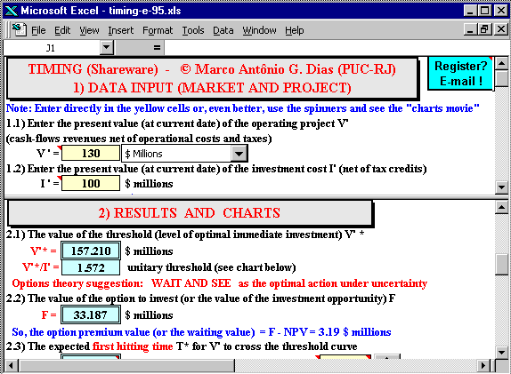
The main screen of the Timing is showed below:
In order to solve the problem, Timing now uses the Bjerksund &
Stensland (1993) analytic approximation.
The adopted approximation is good enough from a practical point of view
mainly for long-term cases typical in real options, and computationally
very fast due its simplicity.
More about the program Timing, including link to download the shareware (totally functional), go to its webpage by clicking the Timing symbol below:

In this case there are two sources of uncertainty. The two stochastic variables are the project value (V) and the development cost of investment (I).
This version uses the fact that the differential equation (from the classic Timing which only V is stochastic) has homogeneity of degree one for the development cost. So that I set:
The partial differential equation for the 2 uncertainties case is:

Where sT is the total volatility explained below.
The figure below shows the screen of the Two Uncertainties version of Timing.
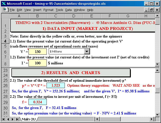
The main difference is the volatility parameters (2 instead 1) and the
correlation coefficient.
With these parameters we get the Total Volatility of the process,
which is given by the equation:

Using this equation and holding sV constant, the effect of both cost volatility and correlation coefficient, is represented by the 3D chart (after see the chart, press back in your browser to return in this point). The introduction of the cost uncertainty doesn't mean that the total uncertainty is higher. For positive correlations, an increase in the cost uncertainty can reduce or increase the total volatility, see chart 2D.
The screen below shows the facilities for volatilities entries (upper panel) and the option chart (bottom panel) for the two uncertainties version of Timing.
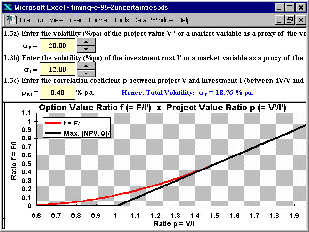
Note that the program points the Total Volatility value, in function of the user entries about the uncertainties (volatilities) of the project value V and investment cost I, and the correlation between these uncertainties.
OBS: Many figures don't show the scroll bars and/or the toolbars, in order to reduce the figure size. To show the scroll bars in Excel, go to menu tools/options/view and mark the to be visible horizontal and vertical scroll bars, and to show the toolbars, go to the menu view/toolbars.
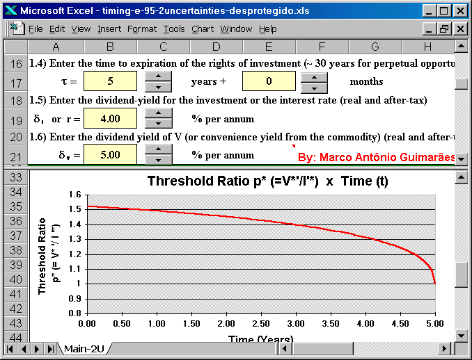
The screen below shows in the upper panel the remaining entries and, in the bottom panel, the threshold chart for the two uncertainties version of Timing.
In this variation, Timing solves an analogous American put option
problem, with both asset value V and exercise price uncertain.
The real option problem is to abandon one project with one important asset
for an alternative use of this asset. There are uncertainty in the valor
of the current asset use and also uncertainty in the alternative use for
the asset.
The table below shows some examples of current asset use and alternative use.
| Asset | Current Asset Use |
Alternative Asset Use |
Market Reference |
| Semisubmersible | Rig drilling in water depth up 400 meters | Floating Production Unit or Drilling Update to 1,000 meters water depth | Rig market value and daily rates, by operational water depth and other rig characteristics. |
| Urban Land (Real Estate) | Restaurant of middle size | Land redevelopment, building a hotel | Restaurant uncertain demand and costs. Hotel uncertain demand and rates. Competition evolution. |
The symmetry between American call and put, eases the adaptation from the early version of Timing.
This Timing-Switch version solves the Myers & Majd (1990) abandon
decision, for the more complex case (two stochastic variables).
See Myers, S.C. & S. Majd (1990): "Abandonment Value and
Project Life" Advances in Futures and Options Research,
vol.4, 1990, pp.1-21
The figure below shows the expected value of two applications of an asset, with the time.
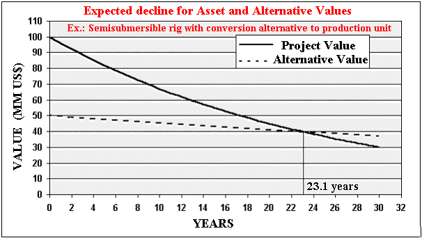
In the chart above, the expected main use value declines with
the physical use, The alternative use is expected to decline slower. The
alternative use declines because the cost to get the same alternative
asset increases with the time. The conversion cost is increasing with the
age of the semisubmersible (older ones needs more reforms).
There are uncertainty in these values (to be estimated by looking the
market) and also correlation (positive) between these values.
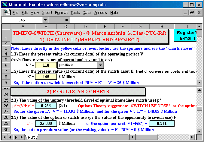
The figure below presents the main screen from the Timing-Switch spreadsheet:
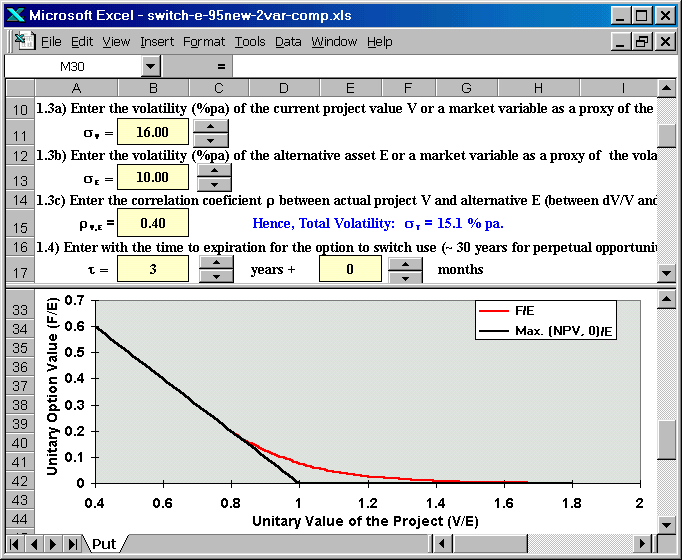
The screen below shows the facilities for volatilities entries (upper
panel) and the option chart (bottom panel) for the switch use option with
two uncertainties. The options chart looks like an American put option.
In the software was used the put-call symmetry, see for example Carr, P. & M. Chesney (1996): "American Put-Call Symmetry" Working Paper, Morgan Stanley & Groupe H.E.C., November 1996, 16 pp. and also McDonald, R. & M.D. Schroder (1998): "A Parity Result for American Options" Journal of Computational Finance, vol.1, no 3, Spring 1998, pp.5-13 (original draft from December 1990).
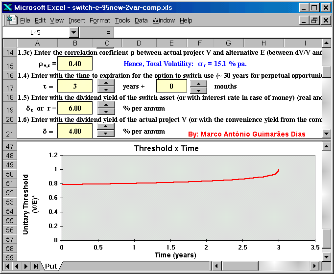
The screen below shows in the upper panel the remaining entries and, in
the bottom panel, the threshold chart for the switch option with two
uncertainties version of Timing. The threshold line follows the American
put option case.
