Quasi-Monte Carlo Simulation

1) Introduction and Motivation.
. . . . . . . . . .Download Excel file QMC_Black_Scholes.xls for European call option with three simulations

2) The Basic Low Discrepancy Sequences (with animation).

3) The Key Role of the Uniform Distribution [0, 1] Numbers and the Moro's Inversion

4) Rate of Convergence and the High-Dimensional Case

5) Halton, Faure, and Sobol Sequences(with animation).
. . . . . . . . . .Download Excel file random_x_quasi-random.xls
. . . . . . . . . .Download Excel file quasi-random-mult_dim.xls

6) A Simple Hybrid Quasi-Monte Carlo Approach (with animation).
. . . . . . . . . .Download Excel file hyb_qr_generator.xls

7) Intuition and Definition of Discrepancy and Low Discrepancy Sequences

8) Regular Grid Updated!

9) Monte Carlo and Quasi-Monte Carlo Internet Links

1) Introduction and Motivation

Quasi-Monte Carlo simulation is the traditional Monte Carlo simulation but using quasi-random sequences instead (pseudo) random numbers. These sequences are used to generate representative samples from the probability distributions that we are simulating in our practical problem.
The quasi-random sequences, also called low-discrepancy sequences, in several cases permit to improve the performance of Monte Carlo simulations, offering shorter computational times and/or higher accuracy.

In reality, the low discrepancy sequences are totally deterministic, so the popular name quasi-random can be misleading.

The essential characteristic of the Monte Carlo method is the use of random sampling techniques to reach a solution of the physical problem.
The use of these sequences of numbers in Monte Carlo simulations can be view in two ways. First, the generation of (quasi or pseudo) random numbers is a way to generate representative samples (a lot of scenarios), to describe the uncertainties of our physical problem through probabilities distributions. We will see that the Uniform [0, 1] distribution permits to generate all the distributions that we need to perform the simulations.
Second, the simulation problem can be viewed as the solution of one (or several) integral, the Monte Carlo Integral. One of first applications of Monte Carlo methods (40's) was the evaluation of complicated integrals (not directly related to the probabilities distributions).
Let us see the Monte Carlo integral in order to illustrate the main characteristic of the quasi-random numbers.

The evaluation of an integral using Monte Carlo simulations is the strongest application of quasi-random sequences, and hence was the initial motivation for research in this area. Quasi-random sequences are more evenly scattered throughout the region that the Monte Carlo integral is calculated, improving the accuracy of the integral evaluation. In order to see this, let the integral of one (any) function f(x) being evaluated using simulation. The idea is to use random points for the numerical evaluation of an integral, that is, using random points to determine the area under the function, see the picture below (based in Press et al., 1992).

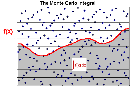
The integral of the function f(x) is approximately the total area times the fraction of points that fall under the curve of f(x). Naturally this method for evaluation of an integral (using "random" points) is competitive only for the multi-dimensional case and/or complicated functions.
Note that the integral evaluation is better if the points are uniformly scattered in the entire area or, for the multi-dimensional case, in the hypercube volume.

The Monte Carlo simulation can be view as a problem of integral evaluation. Recall that to calculate an expected value we have to evaluate an integral (or a summation for discrete probability density case). Ripley (1987, p.119) wrote: "The object of any simulation study is the estimation of one or more expectations of the form Ef(X)". In general, the Monte Carlo method solves multidimensional integrals, and the expression for the Monte Carlo approximation for the multidimensional integral over the unit hypercube is given by:

Referring the above expression, Sobol (1994, p.97) wrote: "...our estimate is an approximation of an integral over the n-dimensional unit cube, derived by averaging the values of the integrand at independent random points G₁, ..., G_N uniformly distributed in the cube". In another topic is discussed the key role of the uniform distribution in the [0, 1] interval generating all the practical distributions that we need.

A finance example: the European call option solved by Monte Carlo simulation is given by the integral below:

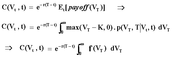
Where E_t[.] is the payoff expectation under risk-neutral (or martingale) measure conditional to the information at the (current) time t; p(V_T, T | V_t, t) is the risk-neutral transition density function of V, which is lognormal for the geometric Brownian motion; V_t is the value of the underlying asset at the (current) instant t; K is the exercise price; T is the expiration time; and r is the risk free interest rate.

In most cases are possible to write the integral in the interval [0, 1] by using a function V = g(u) so that we can use f(u) instead f(V). In other words, writing the integral with the primary uniform numbers that the computer is generating, which are Uniform [0, 1].
The generation of the U[0, 1] numbers is the focus of this page and is very important for the quality of the simulation.

Beyond the integration problem, there are other aspects in the simulation that are important in several cases. For example, the independence along the sample path of a stochastic variable. For problems that we need to simulate the entire path we have a multi-dimensional problem. The number of dimensions is at least the number of time-steps (see more later).
For while, let us see the different ways to generate these random points.

The pseudo-random sequence of numbers looks like random numbers because it looks unpredictable. However, pseudo random numbers are generated with deterministic (explaining the adjective "pseudo") algorithm like the congruential random generator (the most common generator). In addition, the implementation of these pseudo random sequences are, in general, of volatile type in the sense that the seed (initial value of a sequence) depends of an (unpredictable) external feeder like the computer clock. For example, in Excel the function Rand() (a kind of linear congruential generator) returns a different number from U[0, 1] every time you press the recalculation command (F9).
Some risk-analysis software permit the user to choose the seed, allowing to reproduce the exact pseudo random sequence by using the same seed, which can be very useful for the modelers (see Vose, 2000, p.64).

In order to introduce the advantage of the quasi-random numbers over the pseudo random numbers for integration problems, let us to consider the evaluation of the European Call Option by Monte Carlo simulation in order to compare with the very known closed-form formula of Black-Scholes-Merton.
In the following Excel spreadsheet I use a VBA (Visual Basic for Applications) for Excel program in order to evaluate the European call using three types of simulation:
(a) the first simulation using the quasi-random numbers (the van der Corput sequence, see topic 2) and Moro's inversion to get the standard Normal distribution (see topic 3);
(b) the second simulation using the pseudo random numbers from Excel with the Excel's build in function for the Normal inversion; and
(c) the third simulation using the pseudo random numbers from Excel but with the superior Moro's inversion.

Download the compressed Excel file: qmc_black_scholes.zip, with 32 KB (VBA code is not hidden).

Alternative download the non-compressed Excel file: qmc_black_scholes.xls, with 95 KB .

By running the simulations, the reader can verify that in most cases the simulation error with traditional Monte Carlo (pseudo random numbers) is higher or much higher than the error with quasi-Monte Carlo simulation. In many simulations this error is higher by a factor of 10 or more! In some cases the error with pseudo-random sequence is lower, but this occurs by chance in less frequent simulated cases.
Note also that for the quasi-random simulation, a higher number of simulations always improves the accuracy of the simulation.

Even pseudo-random numbers from a reliable random generator, which have "the same relevant statistical properties as a sequence of random numbers" (Ripley, 1987, p.15), in many situations exhibit a too slow rate of convergence for the main problem of a Monte Carlo simulation. The main problem in finance and real options (and in many other fields) is the evaluation of a (multidimensional) integral of a function, e.g., the options payoff function with variable(s) assuming values that obeys some probability density function(s). For this type of application is possible even to sacrifice some statistical properties (like independence), if not required in the practical problem, in name of a faster convergence to the correct value. In this class of problems enters the idea of low discrepancy sequences. For applications requiring the independence property, we have many alternatives such as the use of hybrid quasi-random sequences (see this topic later).

The quasi-random numbers have the low discrepancy property that is a measure of uniformity for the distribution of the points. This is very useful to represent an uniform distribution (and the other distributions, which are functions of the uniform, see later). Mainly for the multi-dimensional case, this is a measure of no large gaps and no clustering of points in the d-dimensional hypercube. We'll see more details later.

The following table illustrates the nice statistical properties of quasi-random sequence (used a van der Corput sequence in base 2, see later the definition) compared with the (theoretical) Uniform [0, 1] distribution, and with two typical pseudo-random sequences (generate with Excel). In the table, the used QR sequence started with 0.5 instead zero, in order to see the minimum number different of zero.

Hence, quasi-random sequence presents a better performance than typical pseudo-random sequences for all four probabilistic moments, indicating that quasi-random sequence is more representative of U[0, 1] than pseudo-random numbers. However, the quasi-random numbers were not developed by statisticians, but by number-theoreticians.
Instead statistics, Quasi-Monte Carlo simulation originates from a different mathematical area: the discipline of Number Theory. Concepts for the measure of dispersion like discrepancy replacing the concept of variance, the use of tools like change of number base (not only from decimal to binary), the use of prime numbers properties, the use of the coefficients of primitive polynomials, and so on, comprise the number theoretic toolkit.
Fortunately some technical details are not necessary to perform a good simulation, if the user owns knowledge of the main concepts and knows when and how to apply these quasi-random sequences. Some formal details are included in a more technical section below, for reference.

There are some problems when using QMC, as pointed out by Morokoff (2000):

First, quasi-Monte Carlo methods are valid for integration problems, but may not be directly applicable to simulations, due to the correlations between the points of a quasi-random sequence. This problem can be overcome in many cases....a second limitation: the improved accuracy of quasi-Monte Carlo methods is generally lost for problems of high dimension or problems in which the integrand is not smooth.

We will discuss later some ways to reduce or by-pass these problems, including the use of hybrid quasi-random sequences.

"Deterministic" Monte Carlo methods started in finance applications with the paper of Barret & Moore & Wilmott (1992) in Risk. Quasi Monte Carlo (QMC) methods began to be popular in finance practice mainly after the work of Paskov & Traub from Columbia University. They used an improved Sobol algorithm for evaluation of derivatives, resulting in the software named Finder, which rose interest of Wall Street firms. This applied research was reported at Business Week in June 20, 1994, in article named "Suddenly, Number Theory Makes Sense to Industry", on the superior results with QMC for high-dimensional problems of derivative evaluation. In the beginning of 90's, the conventional wisdom was that, for the high-dimensional case, QMC was inferior to Monte Carlo.

The basic nice characteristics of low discrepancy sequences are illustrated in the next topic, and later will be more formally defined.

References: There are many recommendable sources in the growing literature on this subject that I used in this page. In general the mathematically inclined reader should consider at least the theory on low discrepancy sequences with the rigor of Niederreiter's book : Random Number Generation and Quasi-Monte Carlo Methods, SIAM, CBMS 63, 1992.
For the practitioner, a good first reading on quasi-random approach is the very didactic and comprehensive article of Galanti & Jung: "Low-Discrepancy Sequences: Monte Carlo Simulation of Option Prices", Journal of Derivatives, Fall 1997, pp.63-83.
A good complement is the paper: Boyle & Broadie & Glasserman: "Monte Carlo Methods for Security Pricing" Journal of Economic Dynamics and Control, June 1997, vol.21, n^o 8-9, pp.1267-1321.
The Dupire's (eds.) book, published by Risk Books, has a collection of many important articles in this subject.
The complete citations/references for quasi-Monte Carlo are found in Monte Carlo bibliography page: the Quasi-Monte Carlo topic.

2) The Basic Low Discrepancy Sequences

The concept of low-discrepancy is associated with the property that the successive numbers are added in a position as away as possible from the others numbers, that is, avoiding clustering (groups of numbers close to other). The sequence is constructed based in the schema that each point is repelled from the others. So, if the idea for the points is maximally avoiding of each other, the job for the numbers generated sequentially is to fill in the larger "gaps" between the previous numbers of the sequence.
The following picture illustrate the "filling in the gaps" dynamic from the van der Corput (1935) sequence in base 2, which is the building block of several important low-discrepancy sequences. This sequence starts from zero, and is confined in the interval [0, 1) with the first 16 numbers (n from 0 to 15) given by:

We use the interval [0, 1) for the sequence definition, closed at zero because this point is included in the sequence, but it is opened at 1 because the sequence never reach the number 1 (although for very large n we get points as close 1 as we like). However, in several applications is common to start from n = 1 instead n = 0 or even to discard the first n' numbers.
Note: I think the sequence is better balanced with the (0, 1) interval instead [0, 1) and, in addition, there are practical problems to work with zero (for example the inversion to obtain the Normal distribution), so that I don't include zero in my set of QR numbers for practical applications.

Clearly the van der Corput sequence exhibits a cyclicality that can be one problem in many applications: it moves upward and falls back in cycles of two (however, a random permutation of the sequence can practically eliminate this dependence, as we see later).
Let us see the static picture for the first 16 van der Corput (base2) numbers. See in the picture below that there are no clustering of numbers in this interval [0, 1).

There are van der Corput sequences for other base of prime numbers. Different bases have different cycle length, the quantity of numbers to cover the interval [0, 1) in each cycle. In base two, the pairs (0, 1/2) and the pair (1/4, 3/4) are the two first cycles.
For other bases this cycle is larger. For example, in base 3 the sequence has power of 3 denominator with length cycle = 3 (e.g., 0, 1/3, 2/3 is the first cycle). It looks like:

0, 1/3, 2/3, 1/9, 4/9, 7/9, 2/9, 5/9, 8/9, 1/27, 10/27, 19/27, .....

The van der Corput sequence, for the number n and base b, is generated through by a three step procedure:

1. The decimal-base number n is expanded in the base b. For example, n = 4 in base 2 is 100 (4 = 1 x 2² + 0 x 2¹ + 0 x 2⁰);
2. The number in base b is reflected. In the example, 001; and
3. Get the reflected base b number. In the example, the base 2 number 0.001 corresponds to the decimal number 1/8, that is, van der Corput = 1/8 = 0.125 (= 0 x 2^-1 + 0 x 2^-2 + 1 x 2^-3).

With two equations we execute these steps. In the first equation we get the inverted base b digits sequences a_j (e.g., for base 2, a sequence of 0's and 1's; for base 3 a sequence of 0's, 1's and 2's, etc.), whereas in the second equation we get the corresponding van der Corput sequence in base b for the required decimal number n:

Where m is the lowest integer that makes a_j(n) = 0 for all j > m.
The reader would be interested in check the base 2 example presented before (the numbers from 0 to 15 in base 2), in order to see that the sequence 0, 1/2, 1/4, 3/4, etc. is reached with these two simple equations. Even easier is to work with the algorithm code that I present below.

The following VBA (Visual Basic for Applications) for Excel code, permits the generation of van der Corput sequence in any base by a user defined function CorputBaseb(b, n), where b is the base (prime number) and n is the number to be transformed (in base 2, for n = 0, 1, 2,... we get 0, 1/2, 1/4, ...). This code is a VBA version of the pseudo-code presented in Wilmott (2001, pp.474-475):

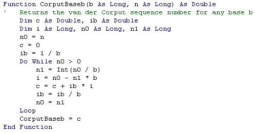
There is a similar VBA code in the book of Jackson & Staunton (2001), but it is for base 2 (not any base) and I prefer to declare the integer variables "As Long" instead "As Integer" used in the book (due the "Integer" format limitation that does not permit to work with a reasonable number of simulations like 40,000 or more).

The next topic presents the explanation about the importance of the Uniform [0, 1] distribution for all simulations, and a relatively new technique to obtain the Normal distribution, which is largely used in finance and needs a special attention. The readers whom know this matter can skip this topic, jumping to item 4, but I recommend to see at least the last table of the section 3 (the accuracy problem with Excel).

3) The Key Role of the Uniform Distribution [0, 1] Numbers and the Moro's Inversion

The Uniform distribution in the interval [0, 1] is, for practical purposes, the only distribution that we need generate for our simulations. The reason is that the samples from the other distributions are derived using the Uniform Distribution. The Uniform distribution can be generate with either pseudo random number or quasi-random numbers, and algorithms are available to transform a Uniform distribution in any other distribution. See, for example, the excellent book of Law & Kelton, 2000, for algorithms using the Uniform distribution to generate the main distributions.

The main and direct way to do this transformation, is by the cumulative distribution function inversion. In order to understand this method let us see the picture below, a cumulative distribution of Standard Normal Distribution, that has mean equal zero and variance equal 1, that is, N(0, 1).

The red line is the cumulative distribution from a Standard Normal Distribution, N(0, 1) , but could be any distribution with known cumulative distribution that the reasoning is the same.
Note that the Y-axis has the same range of the Uniform [0, 1], because [0, 1] is the range where the probability distribution function is defined. More important, the Y-axis space is equiprobable, so we have the Uniform Distribution for the range [0, 1] in the Y-axis. This means that we can associate each y-value drawn from U[0, 1] with any distribution with known cumulative function, including our Standard Normal.
The blue line indicate that with a sample number drawn from the U[0, 1] distribution (in the picture is for y ~ 0.3), we can associate a sample number x for the distribution that we want simulate (in the picture, x ~ - 0.5).

The most important distribution for real options and finance applications in general is the Standard Normal Distribution. The cumulative distribution is the integral of its density function. The density distribution function for N(0, 1) looks like the picture below:

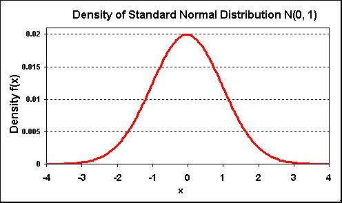
For Standard Normal distribution, the cumulative distribution (cumulative area from the picture above) is:

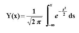
This equation describes the function showed in our first picture of this topic, the cumulative Normal distribution function.

In our simulation problem, we have the Y(x) samples (numbers sampled from ~ U[0, 1]) but we want the corresponding x samples for any distribution, e.g., the Normal distribution. In other words, we want x(Y), the inverse of the cumulative distribution. Hence, given one uniformly distributed sample u we want to obtain the value x(u), that is, the correspondent sample for the desirable probability distribution.

In terms of integral evaluation, let us work the simple example of expected value calculus of a function g(x), which has Normal distribution with density f(x) and cumulative distribution function F(x).
The expected value of g(x) is given by:

However, substituting u = F(x) and letting U ~ Uniform[0, 1], we have the other expected value below.

For example, the integral for the evaluation of an European call option (C) over a stock that values V today (t = 0) with exercise price K, is given by:

Where, being F(x) the standard Normal cumulative distribution function, was performed the substituition u = F(x), so that x = F^-1(u), and u is drawn from the Uniform[0, 1] distribution.
The evaluation by simulation of the above integral with N samples u from the Uniform distribution is performed using the equation:

Let us examine the case of Normal distribution inversion F^-1(u), used in the equation above, due to its importance.

The Moro's Inversion

The known general way to obtain the inverse of a Normal distribution is by using the Box-Muller algorithm (see Press et al., 1992). However, for low discrepancy sequences has been reporting that this is not the better way because it damage the low discrepancy sequence properties (alters the order of the sequence or scramble the sequence uniformity), see Moro (1995), Galanti & Jung (1997), and Jackson & Staunton (2001). In addition, has been reported that the Box-Muller algorithm is slower than the Moro's inversion described below.

The traditional Normal inversion algorithm is given by Beasley & Springer (1977), see Moro (1995). However, this algorithm is not very good for the tails of the Normal distribution. The best way to obtain the inversion from U[0, 1] to Normal distribution is by using an algorithm presented in a famous short paper of Moro (1995). Moro presented a hybrid algorithm: he uses the Beasley & Springer algorithm for the central part of the Normal distribution and another algorithm for the tails of the distribution.

He modeled the distribution tails using truncated Chebyschev series. There is a C algorithm for this kind of series in Press et al. (1992), eqs. 5.8.7 and 5.8.11, mainly. However, the Moro's C code presented in the paper, is directly applied to the our problem of Normal tails.
The Moro's algorithm divides the domain for Y (where Y = uniform sample) into two regions:

1. The central region of the distribution, |Y| 0.42, is modeled as in Beasley & Springer;
2. The tails of the distribution, |Y| > 0.42, are modeled with Chebyschev series.

The Moro's algorithm is very simple, the only job is to write some constants and a few lines of code. The paper of Joy & Boyle & Tan (1996) presents the Moro's algorithm but with some differences, mainly in the constants (apparently, Joy et al. look for more precision with the Chebyschev series), used also in Galanti & Jung (1997). However, the tests that I performed with the original Moro's constants were very satisfactory.
There is a VBA version of this algorithm in the book of Jackson & Staunton (2001): "Advanced Modelling in Finance Using Excel and VBA", which uses the constants from the Moro's original work. With simple short algorithms codes in C and VBA available in the literature, I'll not repeat it here. The interested reader can look directly in these references.

In the next two tables, I present some comparison between the Moro's inversion and the popular Excel inversion. The Excel weakness is noted only in the second table.
In the first following table, I present a result of a limited test (only one quasi-random sample with 1,000 points) about the accuracy of Moro's inversion (using the Moro's original constants) and the inversion using the Excel internal function named NORMSINV(). I used the program Best Fit to check the Normal distribution hypothesis after the inversion (for both inversions, Normal distribution was the best fitting for both chi-squared and A-D tests).
For this test, using a van der Corput quasi-random sequence in base 2, the table shows that both inversions (Moro and Excel) presented practically the same (acceptable) accuracy. In this case, the Excel 97 inversion looks not too bad with QRN as I supposed before, see the results in the table below. Of course, are necessary new tests (including other bases, other sequences, more simulations, etc.) to make a more conclusive statement.

However, the Excel inversion weak point is in the tails accuracy. Let us see the next table, which we take uniform numbers (u) successively closer to zero so that the inverse numbers are successively more negative (in the left tail of the Normal). The "exact" numbers and the idea for this kind of test are drawn from the paper of McCullough & Wilson (2001, p.6). Note the poor performance of Excel in the tails, mainly for u < 0.00001, and I highlight that the last number in the Excel column is not a typographical error!

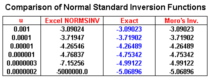
On the contrary, note that the Moro's inversion get the same result of the column "exact" for the precision of 5 decimal digits. This nice performance of the Moro's inversion for the tails can make a significant difference for real options valuation.
The "tail performance" is important for a large number of simulations (so that non-zero low discrepancy numbers get closer of the limits of the interval). For typical (real) options problems, mainly for out-of-money options, the performance of the tails is important because the options exercise is related to occur at the upside (more extreme value), highlighting the weight of the tail in the (real) option value.

Moro's inversion became popular in computational finance community. More recent finance Monte Carlo's books (for advanced finance researchers) also mentioned Moro's inversion: Jackel (2002, p.10) and mainly Glasserman (2004, pp.67-69).

So, I strongly recommend the Moro's inversion instead the Excel build-in inversion for problems that requires some accuracy. McCullough & Wilson (2001) argue that the statistical problems with Excel 1997 were not fixed in the new version Excel 2000.
In addition, perhaps the Moro's inversion is faster, but this test was not performed here.
Last Time News: a small part of the problems (like the big error in the tails) were fixed with Excel XP. However, most problems remains with the XP version: see the paper of McCullough (in the version I read, table 5 showed the tails problem in the Normal inversion).

4) Rate of Convergence and the High-Dimensional Case

The practitioner of simulation is always concerned with the computational time and the numerical error of the simulation. Both are related with the simulation rate of convergence to the true value. The standard error in the simulation can be viewed as the standard deviation of the (random) sample divided by an increasing function of N, the number of simulations or paths.
One way to reduce the error is by looking the numerator, by using techniques of reduction of standard deviation of the sample ("variance reduction techniques"), which are not scope of this section.
The other way to reduce the error is by increasing the number of simulations N. However, there is a trade-off between the computational time and the numerical error. The natural and simplest way to reduce the simulation numerical error is by increasing N, but the computational time increases directly with the number of simulations N.
The rates of convergence to the true value, which are function of N, are given below for both Monte Carlo and Quasi-Monte Carlo simulations:

1. The traditional Monte Carlo (MC) using (pseudo) random numbers, has a convergence rate of only O(N^-½) (think with Central Limit Theorem arguments or see Niederreiter, 1992, Theorem 1.1, p.4). Note that this rate is independent of the dimension d, it depends only of the number of simulations N;
2. Quasi-Monte Carlo (QMC) rate of convergence can be much faster with errors approaching size of O(N^-1) in optimal cases (see e.g. Morokoff, 2000, pp.765-766, and Birge, 1995, p.2).
   One example: for MC is necessary to increase 100 times the number of simulations N to reduce the error by a factor of 10, whereas the QMC requires less (in general much less) that 100 times, and only 10 times in optimal cases;
3. The theoretic upper bound rate of convergence (or maximum error) for the multi-dimensional low discrepancy sequences (Halton and others, see next topic) is of O((ln N)^d/N), see Niederreiter (p.32), where d is the number of dimensions from the practical problem. So, unlike the pseudo-random bound convergence, the quasi-random sequence performance decreases with the dimension d.

The different criteria from items 2 and 3, which can lead to very different results for the rates of convergence of Quasi-Monte Carlo simulations, see the table below (d = number of dimensions; N = number of simulations):

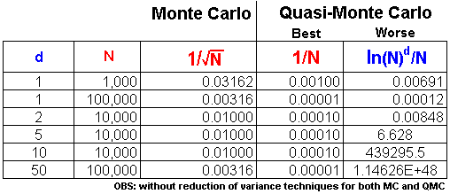
Note that for dimensions higher than 5 in the table, the worst-case for Quasi-Monte Carlo (QMC) is much inferior to the crude Monte Carlo with pseudo random numbers. However the best QMC case is always better than MC. The worst-case bound is not very reliable for practical purposes and, in high-dimensional problems, the reader needs to be aware of the too large required value for N that makes the QMC's worst-case better than the crude Monte Carlo.
Let us to explain better the problem of high-dimensionality.

In finance applications is more common to get results closer of the best rate of convergence than the theoretic worst-case. This occurs sometimes because the use of some technique for the reduction of effective dimension, sometimes because the favorable smooth payoff function and even the discount effect. For instance, in the "performance table" from the Excel file QMC_Black_Scholes.xls, the absolute error function = 7 N ^{- 0.85} (fits with R2 = 0.9995), shows a convergence closer to best case O(N ^{- 1}) than the traditional MC error of O(N ^{- ½}).
Here I refer "smooth function" as, e.g., a function with second derivative Lipschitz-continuous. In this case is possible to show that the worse limit for rate of convergence decreases to O((ln N)^(d-1)/2/N^3/2), see Caflisch.& Morokoff & Owen (1997, p.306) using a hybrid of quasi-Monte Carlo with scrambled (or randomized) nets. The effective dimension of a function is related to its ANOVA decomposition over low-dimensional subspaces.

Boyle at al (1997) wrote: "The reason for the difference..... may be that the integrands typically found in finance applications behave better than those used by numerical analysts to compare different algorithms. Another important consideration is that finance applications typically involve discounting, and this may effectively reduce dimensionality".
Press et al. (1992, p.314) wrote that "Quasi-random sampling does better when the integrand is smooth .... than when it has step discontinuities." and their Figure 7.7.2 suggests than this smoothness effect is stronger for quasi-random than pseudo-random sequences.

Paskov & Traub (1996) found better results for QMC than MC for a problem with 360 dimensions. They evaluated a collateralized mortgage obligation (CMO) using an improved Sobol sequence. Their Sobol algorithm is different of the one reported in Press et al.(1992). They report that the improvements include the development of a table of primitive polynomials and initial direction numbers for dimensions up to 360. Apparently their software (Finder) is available at Columbia University for researchers. The paper of Paskov (1997) has more technical details for the interested reader, exhibiting good performance even for high effective dimensionality.

Another good result for QMC in high-dimensional problems was found by Caflisch.& Morokoff & Owen (1997) also for 360 dimensions, but working with a mortgage-backed securities. They reached good results for QMC methods using techniques like Brownian bridge to reduce the effective dimensionality of the problem.
An introductory and didactic explanation of Brownian bridge with quasi-random sequences is founded at Jung (1998). However, the Brownian bridge can demand additional computation complexity/time (reordering the path) for path-dependent problems, so that it is not a panacea. Willard (1997, p.58) wrote about the Brownian bridge: "Whether this technique or some variation of it can be used to price American or path-dependent derivatives, .... is not obvious".
In most real options problems, we are interested in American options and path-dependence caused by the technical uncertainty, so that we tend to prefer other techniques to avoid multi-dimensional problems.

Caflisch.& Morokoff & Owen (1997) concluded the paper suggesting the use of hybrid Quasi-Monte Carlo, for example using quasi-random sequences for a small number of dominant dimensions and pseudo random (with a good variance reduction technique such as Latin Hypercube sampling) for the remaining dimensions. This point can be exploited by the practitioner. The idea is to get the accuracy of quasi-random approach for the dimensions with higher impact on the results without the disadvantages of higher dimensionality behavior for these sequences.

In a later topic, I will present a different but very simple hybrid quasi-random algorithm, which permits to joint the nice quasi-random vector properties, with the independence property of pseudo random numbers to model the sequence of QR vectors. This approach uses independent (pseudo) random permutations of quasi-random vectors, and apparently avoiding all the problems of high-dimensional degradation of low discrepancy sequences that we discuss above and that we will see better in the next topic with some graphs.

5) Halton, Faure, and Sobol Sequences

The van der Corput sequence is the basic one dimensional low discrepancy sequence. However, How to generate multi-dimensional low discrepancy sequences? This is the object of this topic.
The van der Corput base2 sequence is also the first dimension of the Halton sequence, the most basic low discrepancy sequence of our interest, which can be viewed as the building block of other low discrepancy sequences used in finance.
Halton (1960), Faure (1982), Sobol (1967), and Niederreiter (1987), are the best known low-discrepancy sequences, but this is a growing research area and new sequences are being proposed (see Boyle et al., 1997, p.1296).
The construction process of new LD sequences involves sub-dividing the unit hypercube into sub-volumes (boxes) of constant volume, which have faces parallel to the hypercube's faces. The idea is to put a number in each of these sub-volumes before going to a finer grid.

Faure and Sobol sequence are like the Halton sequence, but with only one base and with a reordering of elements (we see this later). The main difference is related with the multi-dimensional construction of the sequences. The Faure and Sobol sequences change of dimension with a permutation of the quasi-random vectors, that is, reorder the basic QR vector within each dimension.

In our more basic real option problem, with one source of uncertainty, we can think the number of dimensions d as the number of discrete time intervals of one sample path, so d = T/D t, where T is typically the expiration of our real options or the horizon of interest. The number of iterations N is the number of sample paths. So, across the paths at one specific time instant, we want a good uniform sample numbers in order to generate for example a good Normal distribution of a Brownian motion, that probably will result in a Log-normal distribution for prices.
The main challenge for the low discrepancy sequences is to avoid the multi-dimensional clustering caused by the correlations between the dimensions. We wish to generate LD sequences with no correlation for every pair of dimensions (different time instants t and s).
Below are discussed the Halton, Faure, and Sobol approaches, showing the each one has a different way to build a multi-dimensional sequence.

Halton Sequence

The Halton sequence uses one different prime base for each dimension. For the first dimension uses base 2, for the second dimension Halton uses base 3, for the third dimension uses base 5, and so on. Higher base means higher cycle and higher computational time.

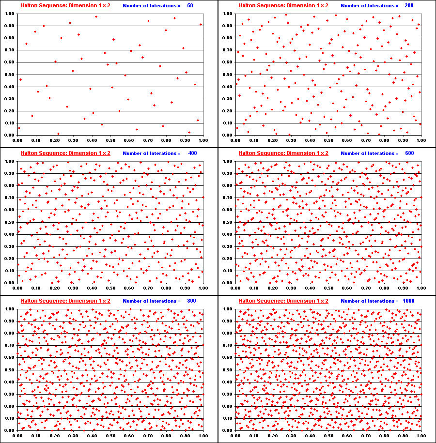
For the case with two dimensions, Halton sequence works with base 2 in the first dimension and base 3 in the second dimension. The two dimensional Halton sequence with 1,000 x 1,000 is displayed below.

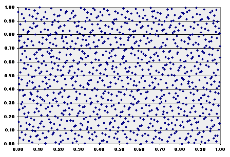
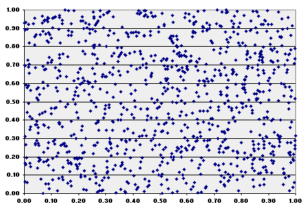
Compare this image with the same plotting but using (pseudo) random numbers of Excel 97:

The following animation shows the "filling in the gaps" process for Halton two-dimensional plotting. See the number of iterations in blue, at the upper right area of this picture (from 50 iterations until 1,000 iterations). Note the nice property of low discrepancy, which increasing finer grid points are generated overlaying the dimensions 1 x 2.

In the previous charts including the animation above, the Halton number sequence started from n = 16 (instead the more common start of n = 1). The sequence preserves its basic properties starting from a different number, so that is not necessary to start from n = 0 or n =1. In addition, there are some advantages to cut the first n* numbers of a sequence to improve the uniformity in higher dimensions, as reported by many authors (e.g., Galanti & Jung, 1997, p.69).

Download: The following Excel spreadsheet permits to compare the quasi-random with random sequences in a two-dimensional plotting. The VBA for Excel code is available without password.

Download the compressed file random_x_quasi-random.zip with 200 KB (contains the Excel-VBA file).

The alternative is to download the non-compressed file version random_x_quasi-random.xls with 805 KB

The major problem for the pure quasi-random sequences is their degradation when the dimension is large. The generation process of uniformly distributed points in [0, 1)^d becomes increasingly harder as d increases because the space to fill becomes too large.
The high-dimensional Halton sequences exhibit long cycle lengths, due the large prime number base. For example, in the dimension 50, is used the base 229, the 50th prime number. The long cycle length means that the high-dimensional sequence needs several numbers for an entire walk in the interval [0, 1).
As pointed out by Galanti & Jung (1997): "This implies that the speed at which increasing finer grid points are generated decreases with increasing dimension"
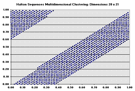
The Halton sequence for 20 x 21 dimensions is showed below and we can see a visible degradation.

The figure below indicates that Halton sequence while still looks uniform in the 2D area, exhibits correlation between dimensions. So, Halton sequence becomes unsatisfactory after ~ dimension 14.

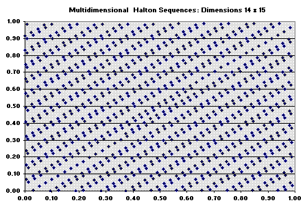
In practice, due the correlation, many people can prefer to avoid the use of Halton sequence for more than 6 or 8 dimensions.

Download: The following Excel with VBA functions and charts, permits the reader to reproduce the results above in multi-dimension by seeing the 2D projections of these dimensions. The VBA for Excel code is available without password.

Download the compressed file quasi-random-mult_dim.zip with 750 KB (contains the Excel-VBA file).

The alternative is to download the non-compressed file version quasi-random-mult_dim.xls with 1,850 KB.

Recall, there are some problems when using QMC, as pointed out by Morokoff (2000):

First, quasi-Monte Carlo methods are valid for integration problems, but may not be directly applicable to simulations, due to the correlations between the points of a quasi-random sequence. This problem can be overcome in many cases....a second limitation: the improved accuracy of quasi-Monte Carlo methods is generally lost for problems of high dimension or problems in which the integrand is not smooth.

These problems have been solved by different means, and later will be presented a simple practical solution with hybrid-low discrepancy sequences. However, let us see some improvements over the Halton sequence with Faure and Sobol sequences.

Faure Sequences

The Faure sequence is like the Halton sequence, but with two differences. First, it uses only one base for all dimensions. Second, it uses a permutation of the vector elements for each dimension.

The base of a Faure sequence is the smallest primer number that is larger than or equal to the number of dimensions in the problem, or equal 2 for one dimensional problem. So, the Faure sequence works with van der Corput sequences of long cycle for high-dimensional problem. Long cycles have the problem of higher computational time (compared with shorter cycle sequences).
As occurred with high-dimensional Halton sequence, there is the problem of low speed at which the Faure sequence generates increasing finer grid points to cover the unit hypercube. However, this problem is not too severe as the Halton sequence. For example, if the dimension of the problem is 50, the last Halton sequence (in dimension 50) uses the 50th prime number that is 229, whereas the Faure sequence uses the first prime number after 50, that is a base 53, which is much smaller than 229. So, the "filling in the gaps" in high-dimensions is faster with Faure sequence when compared with the Halton one.

By reordering the sequence within each dimension, Faure sequences prevents some problems of correlation for sequential high-dimensions that occurred with the Halton sequence. Faure approach makes a link between the low discrepancy sequences theory and the combinatorial theory for the vector reordering.
The algorithm for the Faure sequence uses the two equations given in the topic of van der Corput sequence (see the equations presented before the VBA code), but before using that second equation, there are a combinatorial rearrange of the a_j. This is performed using a recursive equation, from dimension (d -1) to the new dimension d:

In order to use the recursive formulae above, start the first dimension using the van der Corput sequence with the specific Faure's base b, reorder the numbers with the equation above for the dimension d = 2, and so on.
Remember from the basic number theory that mod means modulo and "x mod b" is the remainder from dividing x by b.
Galanti & Jung (1997) use a slight different equation because they use the first dimension (the basic van der Corput sequence) to generate all the dimensions, and the equation above uses the previous dimension (d - 1) to generate the next dimension (d).

There are some variations for this class of sequences. Tesuka (1993) formulated the Generalized Faure Sequence, based on Halton sequence but using polynomials for reordering.

As reported by Galanti & Jung (1997, p.71), among others, the Faure sequence suffers from the problem of start-up (n₀) and, in particular for high-dimension and low values for n₀, the Faure numbers exhibits clustering about zero. In order to reduce this problem, Faure suggests discarding the first n = (b⁴ - 1) points, where b is the base. The start-up problem is reported also for other sequences with the same practical suggestion of discarding some initial numbers from the sequence.

The Faure sequence exhibits high-dimensional degradation at approximately the 25th dimension.
In relation to computational time, as reported by Galanti & Jung (1997, p.80), Faure sequence is significantly slower than Halton and Sobol sequences.

Sobol Sequence

The Sobol sequence, like the Faure sequence, has the same base for all dimensions and proceeds a reordering of the vector elements within each dimension. The Sobol sequence is simpler (and faster) than the Faure sequence in the aspect that Sobol sequence uses base 2 for all dimensions. So, there is some computational time advantage due the shorter cycle length.

However, the simplicity of Sobol sequence compared with the Faure one, ends at this point because the reordering task is more complex. Sobol reordering is based on a set of "direction numbers", {v_i}. The v_i numbers are given by the equation v_i = m_i/2ⁱ, "where the m_i are odd positive integers less than 2ⁱ, and v_i are chosen so that they satisfy a recurrence relation using the coefficients of a primitive polynomial in the Galois filed G(2)" (Gentle, 1998, p.161).

In other words, Sobol sequence uses the coefficients of irreducible primitive polynomials of modulo 2 for its complex reordering algorithm.
There is a C code for an improved Sobol algorithm (due Antonov & Saleev, 1979) in the "algorithm bible" Press et al (1992).

The paper of Galanti & Jung (1997) presents a patient description of Sobol algorithm, including simple numerical examples, and the interested reader should read this paper for an introduction of the algorithm, before look for more advanced sources.

While Sobol sequence "fills in the gaps" at higher rate in high-dimensional problems (due its shorter cycle), there is the problem that at high-dimensions the Sobol points tend to repeat themselves across dimensions, resulting in high-dimensional clustering. The traditional solution is again to discard the first n points. Boyle & Broadie & Glasserman (1995) discard the first 64 points, but it seems arbitrary.

Paskov & Traub from Columbia University used an improved Sobol algorithm for evaluation of derivatives, resulting in the software named Finder. See the article at Business Week, June 20, 1994, "Suddenly, Number Theory Makes Sense to Industry", reporting the superior results with QMC for high-dimensional problems of derivative evaluation.
Apparently they obtained an even better Sobol algorithm version (improvement over Antonov & Saleev, 1979) with specially designed "direction numbers", reaching a better reordering for the Sobol's vectors in high-dimensional problems.

The Sobol sequence (even Antonov & Saleev version) appears to resist more to the high-dimensional degradation. As reported by Galanti & Jung (1997, p. 75): "Surprisingly, the Sobol sequence does not show any degradation through the 260th dimension". So, the Sobol sequence outperforms both Faure and Halton sequences.