Quasi-Monte Carlo Simulation
Continuation

6) A Simple Hybrid Quasi-Monte Carlo Approach

In the practical problem, we need to simulate the sample paths of the underlying asset value (V). At any instant t > 0, we wish that the cross-temporal properties of our sample paths to be, for example, log-normal. The animation below illustrates this problem for a geometric Brownian motion sample-paths.

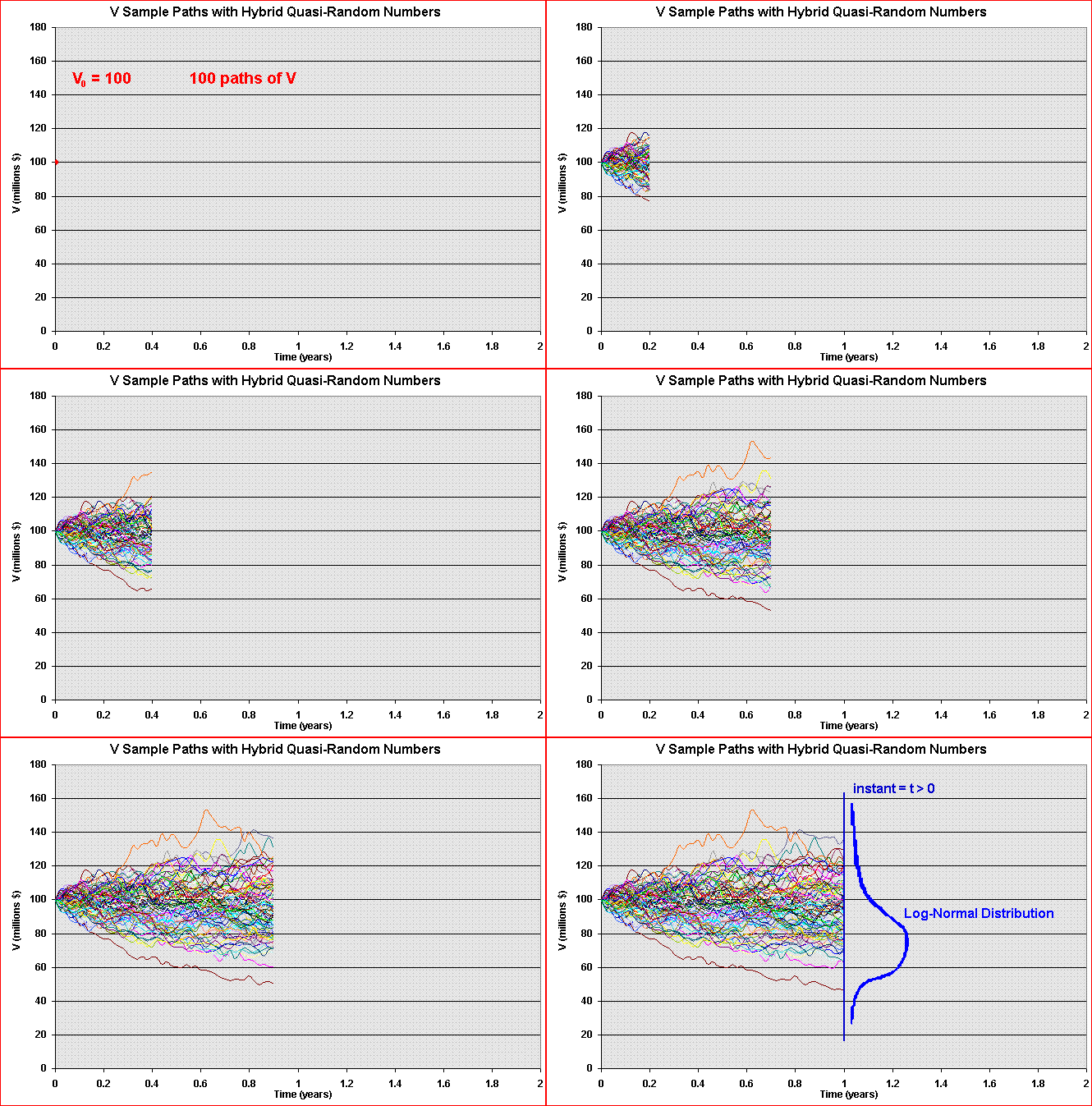
In addition, we need that the increments along the path to be independent. So, the required main property along the time is the independence. Recall the Wiener increment from Brownian motion (and also for other processes of interest like Poisson/jump process) must be i.i.d., that is, independent and identically distributed. So, we need that at any instant t, independent and identically distributed (i.i.d.) samples.

The picture below permits a better understanding. Each column (vector) corresponds to one specific quasi-random sequence. The number of vectors is the number of dimensions D, and can be interpreted, for example, as the number of time-intervals from our discretization of time to the expiration of an option.
The number of elements of each vector, or the number of rows, is the number of simulations N or number of sample-paths.

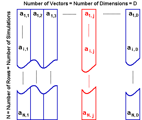
We want that the sequence a_1,1, a_1,2, a_1,3, ......., a_{1, D}, for example, obeys the property of independence.

The simplest way to conjugate the nice cross-temporal properties of quasi-random sequence together with the requirements of independence, avoiding the multi-dimensional degradation of quasi-random numbers, is by a random shift of a low discrepancy vector, so that these points "become mutually independent after the randomization" (L'Ecuyer & Lemieux, 2001, p. 30).

In the picture above, the first vector (column 1) could be the van der Corput base 2 sequence in the original order, whereas any other vector, in general the j-th vector (in red), is a random permutation of the N elements from the original sequence.
In reality, the reader can use the random shifts of the basic low discrepancy vector for all dimensions (including the first one).

The following Hybrid Quasi-Monte Carlo approach is very simple and it is inspired in a Latin-Hypercube technique named stratified sampling without replacement, see Vose, 2000, sections 4.1.2 and 4.1.3, pp. 59-62).
For a problem with D dimensions (e.g., number of periods from a time discretization: D = T/Dt) and N simulations (or paths):

1. Use the van der Corput sequence in base 2 (the simplest LD sequence) vector with N elements as the basic vectors (or for the first dimension); and
2. For each dimension use the van der Corput base 2 vector but with independent random permutations for the elements of this vector.

If N>>D, the independence along the path is reached as a very good approximation, because eases the destruction of the correlation of QR sequences along the path. But even for N = D, the sequence can be sufficiently independent for practical purposes. Fortunately, in practice is more probable to happen N>D or even N >> D.

The random permutation idea is to break the correlations (cyclicality) of the sequence of low-discrepancy vectors. The resulting vector after the permutation preserves its low discrepancy property of an evenly distributed numbers in the interval [0, 1), because the numbers are the same in another order, and in addition the sequence in the same row from the matrix (that is, in the same sample path) gains the property of independence or at least become closer for practical purposes.
So, in the picture above, the sequence a_i,1, a_i,2, ........., a_i,j, ......., a_{i, D}, which provides the quasi-random numbers for the i-th sample path, needs the independence property that the random permutation can provides.

A very simple algorithm for random permutation of a vector is given below in VBA (Visual Basic for Applications) for Excel.
Let X be a vector of low discrepancy sequence (for example the van der Corput base 2) with NI elements, and we need a random swap between the elements X(i) and X(p) for all NI elements. The following algorithm feeds the j-th column of the matrix "Matrix_QR" with a random permutation of the vector X.

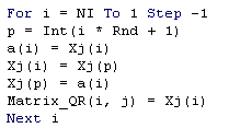
The random permutation here simply uses the Excel/VBA function Rnd, that generates ~ independent U(0, 1) numbers.
Of course, we need to insert the above code into a loop, j = 1 to D, to generate the whole matrix (all dimensions), and also to put the code (given before) to generate the basic vector (non-permuted vector) with the standard van der Corput sequence.

Let us see some charts showing some characteristics of these sequences in multi-dimensional space. The figure below (with 1,000 points) shows that the degradation of low-discrepancy sequence in high-dimensional case is not occurring for hybrid quasi-random sequence (van der Corput base 2).

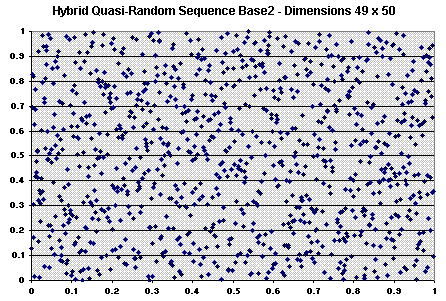
The picture above shows that, in terms of high-dimensional clustering, the hybrid quasi-random sequence is not worse than the pseudo-random sequence in multi-dimensional case. In reality it seems better than pseudo random: compare with the pseudo-random plot presented before and see that the clustering problem is lower. The multi-dimensional sequence being more evenly dispersed in each individual one-dimension, has higher potential to be evenly dispersed at higher dimension if it is possible to eliminate the correlation between dimensions. This job is performed by the random permutation, which makes a random association between the van der Corput numbers for every 2D projection.
We test other pairs of dimensions with similar results, see some of them in the spreadsheet of Hyb-QR Generator.
Most important, by using these hybrid QR sequences we have the guarantee of nice cross-temporal statistical properties: for any time instant t we have a van der Corput base 2 (permuted) sequence, which we see before is a much better approximation for U[0, 1] than the pseudo-random sequence, without the problem of degradation observed in the standard (non-hybrid) quasi-random sequences for higher dimensions.

Download the spreadsheet:

Hybrid Quasi-Random Generator (compressed Excel file [.zip] with 282 KB)

This spreadsheet was written in Visual Basic for Applications (VBA) for Excel 97 (Windows). By clicking in the button, the VBA algorithm will ask you about the number of simulations (default is 1,000) and the number of dimensions (default is 50), will clear the previously plotted numbers, and will write the HQR numbers in the sheet. In my personal computer (Pentium III, 1 GHz), the calculation time plus the writing time take about 4 seconds for the default N and d. This time is spend mainly in writing in the spreadsheet (HQR calculation take less than the half-time) and to update the charts. There are 4 charts in the spreadsheet, plotting two different dimensions in each chart (like the chart above).
In this spreadsheet, the limit of the number of dimensions is the limit of columns in Excel (so up ~250 dimensions is possible), and the limit of the number of simulations is the limit of rows in Excel (~ 65,500).
The first column (or first vector) generated by this spreadsheet is the pure (non-hybrid, ordered) van der Corput sequence. The presentation of the pure vector in the spreadsheet is important for didactic reasons. In practice most users will use only randomly permuted vectors in order to get a more "random" sequences, so that the users can prefer to discard the first column for the applications. The Timing software do discard the first column, using only hybrid quasi-random vectors.
The VBA code is password-protected in this case, but the spreadsheet has all functionality. The reader with knowledge of VBA and with the previous specific VBA codes for Halton sequence and for random permutation of vector elements, can build his/her HQR Generator.

For several (non-correlated) stochastic processes, one idea is to use a type of quasi-random vector for each process, with independent random permutations along the path. For example, using the van der Corput base 2 and its random permutations to simulate the stochastic process of the value of project V and a van der Corput base 3 and its random permutations to simulate the stochastic process for the investment cost of the project.
This is (roughly) the idea of Latin Supercube presented in Owen (1998).

Independence Evidence and Statistical Tests for Independence

The only remaining important check for the quality of our very simple hybrid quasi-random numbers is the test for independence along the dimensions (along the path).
The no clustering looking exhibited in the last picture above (and other plotting between high-dimensional projections, not showed) is a good indicator of no correlation among dimensions for this hybrid quasi-random sequence. For example, if successive uniform vectors exhibit positive correlation, the unit square (2D projection) will exhibit clustering around the southwest-northeast diagonal.
This is exactly the idea of the chi-square test to higher dimensions, also called serial test, see Law & Kelton (2000, p.419), which is an indirect test of independence for the vectors of uniform numbers.
Chi-square test has been rejecting some popular random number generators. For example, Walker (1998, see Chi-square Test) reported that the standard Unix rand() function was not approved by the chi-square test of randomness (the output of that function was classified as "almost certainly not random").
The application of chi-square test for hybrid quasi-random sequences was performed for several sample-paths using the NAG Statistical add-in for Excel (http://www.nag.com/) . For all tests the null hypothesis of independence was not rejected at significant level of 0.10, with probability higher than 0.90.

Other common test for independence of generated random numbers is the runs test or runs-up test (see Law & Kelton, 2000, pp.419-420, or Banks et al., 2001, pp.270-278, or even Knuth, vol.2, 1998, pp.66-69). The statistic for comparison is again the chi-square (see Knuth).
Law & Kelton (2000, pp.419-420) provide a simple and didactic numerical example for this test.
The textbook of Banks et al (2001, pp.270-278) provides a didactic and more detailed discussion with several numerical examples, and it is the best choice for understanding the ideas and variations of this test.
Tables for the runs test are presented in Zwillinger & Kokoska (2000, pp.354-364).
Using again the NAG Statistical add-in for Excel, I ran a runs test for one hybrid quasi-random sample-path (50 numbers), resulting in a significance of 0.69325 for a test-statistic of 0.39445. This is a much better than the result of the non-randomized van der Corput base 2 sequence (from n = 1 to 50), with a significance of 4.25 x 10^-11 for a test-statistic of 6.59500, reflecting the cyclicality of the sequence. Hence, this test is a good indicator that our hybrid quasi-random sequences have the independence property.

I did also some preliminary tests using the software Eviews. First, I choose one hybrid quasi-random path (50 values or dimensions) and I did the conversion from U[0, 1] to N(0, 1), that is, using the Moro Normal Inversion I get the standard Normal (mean zero and unitary variance) correspondent values along the path. After this I test this series in order to check if the white noise hypothesis (Normal i.i.d.) is a good approximation.

The picture below shows the correlogram of a N(0, 1) sample path build up with the hybrid quasi-random approach. The visualization of the usual default limits (from the software Eviews) indicates no significant correlation in the path.

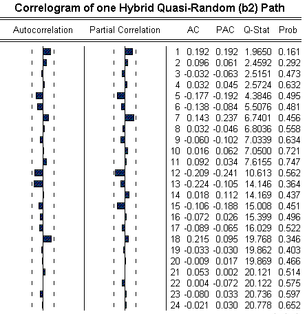
In addition to the indications of no autocorrelation (both in the picture above and the no clustering feature in the high-dimensional unit square), and the preliminaries tests reported before, I ran the test for independence default of the Eviews, the BDS (Brock & Dechert & Scheinkman) test, which is an improvement for financial time series in relation to other older tests like Ljung-Box, Box-Pierce, Turning Points, and so on. The BDS statistics with bootstrap needs to be close to zero in the null hypothesis of BDS test. In the preliminary tests I found BDS statistic close to zero (the worst case was BDS = - 0.053910 and the best case was BDS = - 0.000774).

Other tests can be performed in order to corroborate the independence approximation. In general is expected that for large N relative to the number of dimensions d (that is N>>d), the independence approximation is more reasonable.

There are other randomized (or hybrid) quasi-random approaches, which are more complex but aiming better results. For example, Ökten (see his website in the page of links) uses random sampling from low discrepancy sequences, but he mentions two other hybrid QMC, namely, Owen, using randomized nets and sequences, and Tuffin, using random shift.
A more recent paper of Tan & Boyle (2000), analyzes the Owen approach of randomized QR sequences, suggesting an improvement for high-dimensional cases, exhibiting better performance than both crude MC and classical QMC methods.

7) Intuition and Definition of Discrepancy and Low Discrepancy Sequences

First the intuition: imagine we have 1,000 points and a box that is a cube with volume equal one. How we distribute the 1,000 points in the cube space, so that any (sub) volume in the box that we sort has a number of points in it that is proportional to the respective volume? This is a classic problem in measure theory solved by the mathematician Roth. He formulated the problem of low discrepancy. Discrepancy is related the worse deviation of the percentage of points in any sub-volume (or sub-rectangle, if you imagine a thin slice in the space) in relation to the exact percentage of points for a perfect evenly distributed points. Working with unit hypercube, we work directly with percentage of unit volume for sub-volumes.

Discrepancy measures the extent to which the points are evenly dispersed in the unit hypercube. Assume a d-dimensional simulation and imagine a d-dimensional unit hypercube (volume = 1) and a set of points scattered through out this volume. Let R be a subrectangle, that is, a thin slice of the unit hypercube [0, 1)^d, with volume v(R). The discrepancy of a sequence {x_n} with N points is defined by:

For all subsets R of the d-dimensional unit hypercube. Note that this concept is associated to the worst-case among clustering and spatial gaps.

We are interested in some sequences with special properties. A uniformly distributed infinite sequence in the d-dimensional unit hypercube has the property:

The equation means that this kind of sequence has its discrepancy reduced to zero for a very large number of simulations, so the number of simulations improve the performance of the sequence.

A low discrepancy sequence is one satisfying the upper bound condition:

The constant K depends of the sequence and even of the dimension, but does not depend of N. Researchers are looking for new sequences with low constant K even for high-dimensional cases.
A numerical example using Halton sequence for a three dimensional integration of an exponential function is presented in the textbook of Thompson (2000, pp. 50-51). The resultant value for that constant K was about 6.5.

8) Regular Grid

The regular grid of points (or lattice methods) seems be an intuitive alternative for the integral evaluation, instead the use of random or quasi-random points. For one to few (3 or 4) dimensions this alternative works acceptable or not worse than random sampling. For dimensions higher than 4, regular grid is not practical. This is explained below.

The points in the regular grid are centered into each cell of the grid. The picture below illustrates the regular grid.

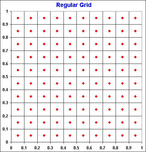
There are three problems for the use of regular grid for evaluation of integrals. First, the problem of dimensionality. Second, is not possible to use regular grid incrementally. Third, the concavity bias.
The first two problems are analyzed in Tavella (2002, pp.105-106), whereas the three problems are analyzed in Dupire & Savine (1998, pp.52-54). These problems are explained below.

The problem of dimensionality: following Tavella (2002) in order to get an intuition, first a favorable case in one dimension. Imagine the evaluation of an European call option by simulation. In this case we need only to simulate at t = T (expiration).
The integral for the evaluation of an European call option (C) over a stock that values V today (t = 0) with exercise price K, is given by:

Where, being F(x) the standard Normal cumulative distribution function, was performed the substituition u = F(x), so that x = F^-1(u) (recall the topic 3, "The Key Role of the Uniform Distribution..." discussion). Since u is a number from the interval [0, 1], in the regular grid approach, instead the random number from an Uniform distribution U[0, 1], it uses equally spaced numbers in this interval so that Du = 1/N, where N is the number of divisions of the grid (N corresponds to the number of simulations in the random sampling case).
This is illustrated in the discretized equations below, being the first one more general - usable for random sampling - and the second is for regular grid (making Du = 1/N):

For this one-dimensional case, the regular grid is very efficient. Tavella (2002, p.105) reports that using only four equally spaced points, the value of a call is found with three digits of accuracy!
However, Tavella adverts that "the number of data points needed to sample from grids explodes like N^d, where N is the number of points per dimension and d is the number of dimensions". This is a big obstacle for the use of regular grid for multi-dimensional problems. Tavella recalls that this difficulty is of the same type faced by the finite differences approach.

Dupire & Savine (1998, p.53) and also Jäckel (2002, p.8) pointed out that the rate of convergence of the regular grid schema is of order O(N^-2/d), where N is the number of simulations and d is the number of dimensions. Recall that the relative error in the crude Monte Carlo is of order O(N^-1/2). Hence, compared with the crude Monte Carlo, regular grid (lattice methods) presents higher error for dimensions d > 4.
This conclusion is not intuitive at first sight, and a (partial) explanation is given below.

The lack of incrementally problem: This is explained by Tavella who says: "It is not possible to incrementally enlarge the size of the grid and at the same time keep the grid uniform. This means that with a uniform grid approach it is not possible to have a termination criterion that can be invoked incrementally. This is a very serious limitation.".
It is easy to see that the quasi-random approach does not have this kind of problem. In order to visualize this in two dimensions, take a look again in the animation on the Halton sequence.

Dupire & Savine (1998, p.54) on this problem wrote: "Low-discrepancy sequences fill the space in an additive way, which means that the (N+1)th point does not modify the position of the first N points (sequences tend to place it in the centre of the biggest gap left by the previous points). This property is not satisfied by other structured schemes such as the regular grid... and presents obvious computational advantages".

The concavity bias: The problem with regular grid is that the concavity of the function being evaluated produces a bias on the subdivisions of the regular grid above, and the errors add up throughout the simulation space.
Dupire & Savine (1998, p.53) wrote: "The integral of a globally convex function is undervalued, while the integral of a concave function is overvalued.". The picture below, a zoom into a single cell of the grid above, permits a better understanding of this affirmative.

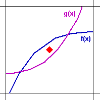
Note that the area under the convex function (in violet) g(x) line is greater than the area above the violet line, but the point from the regular grid schema falls above the line. This undervalues the convex function (recall our discussion of the Monte Carlo integral in the introduction of quasi-random simulation). In case of random sampling (instead the regular grid sampling), a random point in this cell has even more chance to fall under the violet line than above (the chance is the fraction of the area below the line).
For the concave function (in blue) f(x), the opposite occurs: the point from a regular grid schema falls under the blue line even being the area under the blue line lower than the area above the blue line. Again, a random point has good chances to fall above the blue line. In this case even higher probability (proportional to the fraction of the area) to fall in the higher area region (here above the blue line).

Dupire & Savine (1998, p.53) wrote: "regular grid generates small errors that add up, whereas random sampling generates big errors that cancel on average". This is the intuition for the apparently paradoxical advantage of random numbers over the regular grid in high-dimensional case, which the bias adds up throughout the dimensions.
The authors analyzed an alternative named "uniform sampling with antithetic noise" (UWAN) which they tried to link the regular grid advantage with a random noise, in order to cancel the errors. However, for high dimensions the power of UWAN deteriorates (as d grows, the UWAN is reduced to a standard antithetic random sampling).

However, Dupire & Savine pointed out that "low-discrepancy sequences are not able to integrate convexity correctly".
I think that the problem of function concavity is (much) more severe for regular grid schema than for the "regularity" of low-discrepancy sequences.
In addition, the practitioner can design thinner grids for the regions where the function curvature is higher. In real options problems for example, the threshold line (free-boundary curve) curvature is higher near the options expiration than the region far from the expiration.