![]()
![]()
Stochastic processes concern sequences of events governed by
probabilistic laws (Karlin & Taylor, "A First Course in
Stochastic Processes", Academic Press, 1975).
In finance and economics problems, sequences of events take time, so we
can think on random events along the time. Let us see a little more formal
definition.
"A stochastic process X = { X(t), t
![]() T } is a collection of random variables. That is, for each
t in the index set T, X(t) is a random variable. We often interpret t as
time and call X(t) the state of the process at time t" (Ross, 1996,
p.41).
T } is a collection of random variables. That is, for each
t in the index set T, X(t) is a random variable. We often interpret t as
time and call X(t) the state of the process at time t" (Ross, 1996,
p.41).
The index set T can be countable set and we have a discrete-time
stochastic process, or non-countable continuous set and we have a continuous-time
stochastic process. Any realization of X is named a sample path,
which can be discrete or continuous.
Although in most applications the index set is simply a set of time
instants tk, for the case of technical
uncertainty it is not true. Imagine a sequential investment in
information process to determine the volume of a oil reserve. In the
sequence of information revelation random variables (sequence of
conditional expectations with new information - a Doob type
martingale) the index set is a sequence of investments in information
(a set of events, being each event one investment in information).
That is, they are event-driven processes (evolve only if a new
investment in information is performed) and not time-driven processes
as most stochastic processes, which evolve with the pure passage of time.
The former is a special case analyzed in a separated
section.
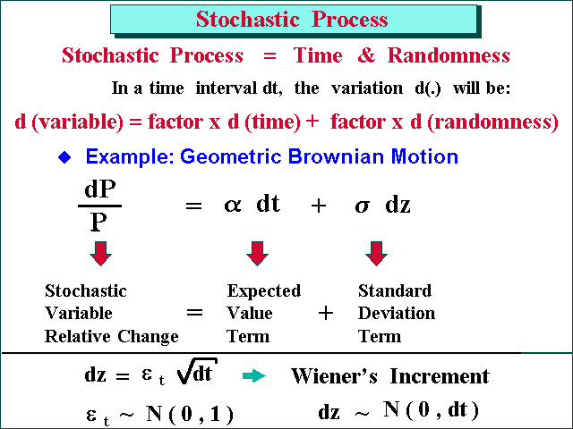
Following Dixit & Pindyck's textbook (p.60): "Stochastic process is a variable that evolves over time in a way that is at least in part random". So, a stochastic process means time and randomness in this section.
For example the temperature in Rio de Janeiro is partly deterministic
(lower temperatures are expected at night and in the winter), and partly
random. In 1997 until October, the hottest 1997 day in Rio de Janeiro
occurred in the winter!
Curiously, the same occurred in 1999, until September, the hottest 1999
day in Rio de Janeiro was September 8 (Winter in Brazil).
So, there are factors that make the temperature unpredictable.
In most cases, a stochastic variable has both a expected value term
(drift term) and a random term (volatility term).
We can see the stochastic process forecasting for a random variable X, as
a forecasted value (E[X]) plus a forecasting error, where error
follow some probability distribution. So:
X(t) = E[X(t)] + error(t)
The figure below presents the idea, a popular example, and brings the concept of increment (in this case the Wiener increment).
Below is presented some general concepts of stochastic processes.
Lévy processes are stochastic processes with
stationary independent increments and continuous in probability.
Stationary increment property means that the probability distribution for
the changes in the stochastic variable X, depends only on the time
interval length.
Independent increments means that for all time instant t, the increments
are independents.
The two most basic types of Lévy processes are Wiener processes and
Poisson process.
Markov processes have the following property: given that
its current state is known, the probability of any future event of the
process is not altered by additional knowledge concerning its past
behavior.
In a more formal words, the probability distribution for xt + 1
depends only of xt, and not additionally on what
occurred before time t (doesn't depend of xs, where
s < t).
Itô process is a generalized Wiener process. A Wiener process is also a special case of a strong diffusion process that is a particular class of a continuous time Markov process (see Merton, Continuous Time Finance, 1990, pp. 121-122 and note 3).
A continuous time Wiener Process (also called Brownian motion) is a stochastic process with three properties:
The Itô process (or Generalized Wiener Process) for the value of a project V is:
dV = a(V, t) dt + b(V, t) dz
The generalized term is because the drift a(V, t) and the variance b(V, t) coefficients are function of the present state and time.
The integral version for this equation, is the following stochastic integral:
As an illustration of stochastic integral, consider the following mean-reverting process (arithmetic Ornstein-Uhlenbeck) process:
dx = h (m - x) dt + s dz
Where m is an equilibrium level which the process reverts and h is the reversion speed. The value of the stochastic process at a future date T, that is x(T), given the starting value x(0), is:

See a discussion of this case in Bjerksund & Ekern (1993).
Point process is a stochastic process whose realizations
are, instead continuous sample paths, counting measures.
Any counting process which is generated by an iid (independent
identically distributed) sum process (Tn) is called renewal
counting process.
The simplest and most fundamental point process is the Poisson process, also referred as jump process in the financial literature.
The Poisson process is a counting process in which interarrival
times of successive jumps are independently and identically distributed
(i.i.d.) exponential random variables.
The Poisson process is an example of renewal counting process.
Homogeneous Poisson Process has the following three properties:
Which is a Poisson distribution with parameter l
t.
A curiosity: the Poisson distribution tends to the Normal
distribution as the frequency l tends to
infinite. So, a Poisson distribution is asymptotically Normal.
A Nonhomogeneous Poisson Process is more general than
the homogeneous one: the stationary increment assumption is not required
(remain the independent increment assumption), and the constant arrival
rate l of a Poisson process is replaced by a
time-varying intensity function.
For an introduction about nonhomogeneous Poisson processes, see
E.P.C. Kao, Chapter 2 ("An Introduction to Stochastic Processes",
Duxbury Press, 1997).
Compound Poisson Process:
Let Fi be a sequence of
i.i.d. (independent and identically distributed) random variables. These
identical probability distributions can be interpreted as the jump-size
distributions. Let N(t) be a Poisson process, independent of
Fi.
The following process is called a Compound Poisson Process:

The sum of two independent compound Poisson processes is itself a
compound Poisson process.
A jump is degenerate when the variable can only jump to a fixed value, and remains in this value. Example: the case of "sudden death" process which the variable drops to zero forever (see Dixit & Pindyck, chapters 3 and 5, for some applications).
Interesting that the combination of Poisson processes with Brownian
motions is related to Lévy process. Karlin & Taylor ("A
Second Course in Stochastic Processes", Academic Press, 1981), p.432,
states "The general Lévy process can be represented as a sum
of a Brownian motion, a uniform translation, and a limit (actually, an
integral) of a one-parameter family of compound Poisson processes, where
all the contributing basic processes are mutually independent".
In the sample paths of Lévy processes, the large increments or "jumps"
are called "Lévy flights"
A general Lévy process (that is, not Gaussian like Wiener process) has been object of recent research for the financial options and real options. Examples:
See also theory on optimal stopping for Lévy Processes, closed form for perpetual options, and more in:
In order to download the papers above and learn more on Lévy Processes, go to Prof. Mordecki's website, with papers and presentations.
![]()
Also named jump-diffusion processes, a combination of Itô process with a Poisson process, (a processes mix, continuous with discrete), can be described by the following equation:
dV = a(V, t) dt + b(V, t) dz + V dq
Where the terms are as before but the additional dq is a Poisson term defined by:
dq = 0 . . . . . . . with probability 1 - l dt
dq = F - 1 . . . . . . . with probability l dt
The processes dz and dq are independents.
In the above equation, l is the arrival rate of jumps and F is the jump size probability distribution (the jump size/direction can be random).
In case of jump, the stochastic variable V will change from V to VF
The other equivalent (perhaps clear) format to write this jump-diffusion equation is:
dV = a(V, t) dt + b(V, t) dz + V (F - 1) dq
Where the Poisson term dq is here defined by:
dq = 0 . . . . . . . with probability 1 - l dt
dq = 1 . . . . . . . with probability l dt
The integral version for this equation, is the following stochastic integral:

Where N(t) is the number of jumps until the instant t, drawn from a
Poisson distribution.
In most cases:
a(V, s) = drift (= a V, for the Geometric
Brownian case; but could be a mean-reverting drift, which has other
format)
b(V, s) = s V
c(V, s) = V (F - 1)
For the case of Geometric Brownian with Poisson-jumps, the logarithm version (v = LnV) of the stochastic equation is:
d(LnV) = (a - 0.5 s2) dt + s dz + Ln(F) dq
The returns generated by a jump-diffusion process are not normally
distributed, presenting fatter tails.
The following picture resulted from a jump-diffusion simulation for a
logarithm of a price (with jumps-up and jumps-down):
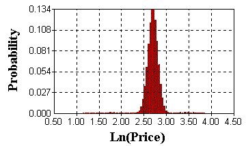
When comparing with a normal distribution (from pure Brownian
processes), the above distribution presents higher peak and consequently
fatter tails.
Even being small tails (low probability density), its size could mean
large losses (or large gains) for financial or real derivatives. So, jumps
can be very important.
In the picture there are some samples near 1 (so, prices near zero) and
samples near 4 (prices near 54), although most values are between 2.5 and
3 (prices in the range 12-20).
For petroleum applications, the most relevant jump-diffusion process is
a combination of mean-reversion (continuous process) with jumps (discrete
Poisson process).
For real options applications, in general we are interested in low
frequency large jumps (rare large jumps), which can be jump-up
or jump-down. The chart below presents sample paths from a
mean-reversion with low frequency jump model. In this case, the initial
price is 15 $/bbl and the long run mean value (which the price reverts) is
also $15/bbl (imagine a heavy oil, with lower long run price). The
simulation is for three years ahead.
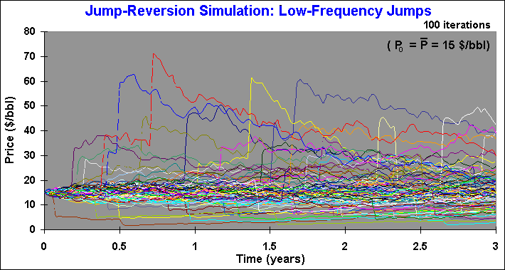
The chart above uses l = 0.2 per year, meaning an average of 20 sample paths with jumps from 100 sample paths, each year. In the chart, some jumps are visible and others the jumps are smaller and their sample paths are hidden by the continuous sample paths near the long run mean price (15 in this example). Sometimes, in the same sample path, occurs another jump few weeks after a jump.
Less realistic for oil prices is the combination of large jumps with
high frequency of jumps arrival. Less realistic because the idea is
associate jumps with "abnormal" rare news (very important news),
whereas the continuous process (mean-reversion) is associated to the "normal
news" (this is the Merton idea, from a famous 1976 paper).
The chart below presents the simulated sample paths from a mean-reversion
with high frequency jumps l = 1 per year).
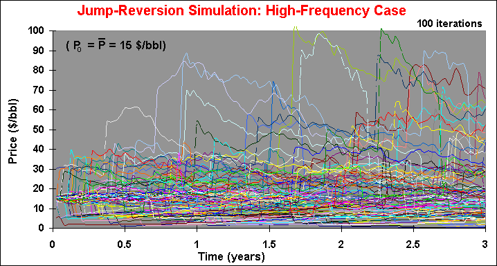
Hence, we are looking for large jumps consistent with rare abnormal news. With this focus, the frequency of jumps is a number like one for each 5 years (l = 0.2 per year), as in the first sample paths chart (low-frequency jumps).
The problems with jump-diffusion processes are the parameters estimation and the portfolio hedging. See a discussion in the section of Mean-Reversion with Jumps Models. Even with some practical problems, the jump-diffusion process is perhaps the best bet for most uncertainty of commodities prices.
![]()
This section follows mainly the paper of Ball & Torous ("A
Simplified Jump Process for Common Stock Returns", Journal of
Financial and Quantitative Analysis, vol.18 (1), 1983). However, the
reader can also found many books on probability and stochastic processes
which discuss the construction of the Poisson process starting from a
sequence of Bernoulli distribution variables.
The main advantage of the Ball & Torous insight is related with the
empirical job of estimating parameters from jump-diffusion processes, as
we will see in this section.
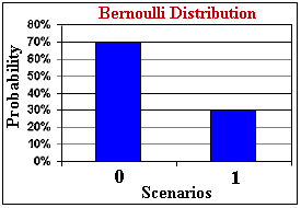
The Bernoulli distribution, Be(p), is the simplest distribution in the Theory of Probability. It is a univariate discrete distribution with only two discrete scenarios, one scenario with value zero (failure) and the other with value 1 (success). The unique parameter p (probability of the scenario with value 1) is also the mean of this distribution. The figure below illustrates the Bernoulli distribution for p = 0.3 (or 30%).
A typical Bernoulli distribution in petroleum is the chance factor (or probability of success) to find petroleum when valuing a wildcat drilling investment. Bernoulli distribution is the building block to construct many other distributions in probability, such as binomial, geometric, hypergeometric, negative binomial, and Poisson. The connection with the Poisson process is the object of this section.
Here we will use the Bernoulli distribution to set the occurrence
(scenario X = 1) or lack of occurrence (scenario X = 0) of a jump
in a stochastic variable.
Let us first define the concept of a function f being o(h)
("order h"). The function f is called to be o(h) if:

Now, let us develop the link between Bernoulli and Poisson distributions. Let N(t) be the number of events (jumps) arriving in a time interval of length t. Denote n a positive integer, and consider the subdivision of the time interval (0, t) into n equal subintervals of length h so that h = t / n. Let Xj be the number of jumps (events) that occur in subinterval j. By the stationary independent increment assumption:

This is a counting process summing n i.i.d. random variables with the properties:
If n is a large number, the probability of a jump in this subinterval j
is negligible so that each Xj is approximately a Bernoulli
random variable with parameter l h =
l t / n.
This is an alternative way to define a Poisson process which is
equivalent to the previous definition as we will see below.
Being a sum of independent and identically distributed Bernoulli random variables, N has a binomial distribution. The binomial distribution is given by:

Where k = 0, 1, 2, ...
What's happen if the time subinterval is very small, that is, if n tends
to infinite? The binomial distribution tends to the Poisson distribution
with parameter l t. See below:

For the proof of the above limit, see for example Ross ("A First
Course in Probability", 5th edition, 1998, p.154).
As Ball & Torous pointed out, this is the standard construction of the
Poisson process.
Let us assume now that the time interval t is very small. Consequently,
N is well approximated by the Bernoulli random variable X with parameter
l t.
That is, X ~ Be( l t) given by:
The main practical feature of the Bernoulli jump process is that over a
period of time t (e.g.: 1 day), either no abnormal (jump) information
occur or only one relevant abnormal (jump) information occur.
The advantage of this approach is related with the empirical analyses, as
developed by Ball & Torous. Under regular conditions, parameter
estimates are asymptotically unbiased, consistent, and efficient, being
obtained economically using maximum likelihood estimation.
In addition, the statistical test of the null hypothesis
l = 0, can be implemented.
Ball & Torous implemented both the method of cumulants and maximum likelihood estimation, with better results for the latter. In addition, their hypothesis tests showed the presence of jumps in most stock returns time-series.
The parameters from the Poisson-Gaussian process of mixing jump process with a geometric Brownian motion (GBM), can be estimated with a Bernoulli mixture of Normal densities, as performed by Ball & Torous. Over t = 1 day, the stock return density f(x) is in this case:
f(x) = (1 - l) F(a, s2) + l F(a, s2 + z2)
Where Ball & Torous assume the mean jump size equal to zero, jump
size variance of z2, and daily
volatility of the GBM equal to s. The above
density expression can be interpreted as the convex combination of two
Normal densities one of them with the variance augmented by the jump-size
variance.
Assuming n daily stock returns x = (xi, i = 1,
2, ...n), and denoting by g
the vector of parameters to estimate (l, s, z, a),
the logarithm of the likelihood function L(x;
g) is:

So, the empirical job of maximum likelihood estimation consists in
maximizing the above function for the four parameters. This is performed
by deriving the above expression in relation to each one of the four
parameters to estimate and equaling these equations to zero. The
sufficient conditions for the existence of maximum require that the matrix
- H(x; g) be positive
definite, where H(x; g) is
formed by the second derivatives of the ln L(x;
g) with relation to the parameters to
be estimated.
With this procedure, Ball & Torous got good empirical results for
stock returns.
![]()
Itô's Lemma is the main tool of the stochastic
calculus. Itô's Lemma in the stochastic calculus is like the Taylor
expansion for the ordinary calculus.
The following example illustrates the comparison and the basic idea of Itô's
Lemma. Suppose an option value F(V, t) and we need the value of dF.
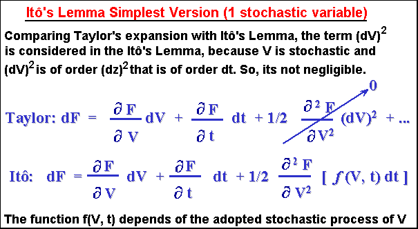
The Itô's Lemma is largely used to construct differential
equations for a function (like options) of stochastic variable(s). Imagine
in the above example, V is a project value (after investment) and F is a
derivative of V, F is a real opportunity to invest in V (that is, F is a
real option).
If you describe the stochastic process for V, the same you can perform for
F by using the Itô's Lemma for dF.
When building a riskless portfolio (nowadays largely used approach based
in arbitrage), is necessary to know the value of the option incremental
value dF. The Itô's Lemma is the way.
Another application. Several books bring the proof, by using the Itô's
Lemma, that if
dV/V = a dt + s
dz
The function v = ln(V), follows:
dv = d(lnV) = (a - ½
s2) dt + s
dz
So, we get a process for v, but with parameters of other process V.
The key feature on the Itô Lemma is that, the square of the Wiener increment is not negligible. More, it is deterministic! Let us prove that (dz)2 = dt:
(dz)2 = (e (dt)0.5)2; where e ~ N(0, 1), the standard Normal distribution.
(dz)2 = e2 dt
But Var(e) = 1 by definition of e. So,
Var(e) = 1 = E[e2] - (E[e])2
The last term is zero by definition of e. So, E[e2] = 1. So,
E[(dz)2] = E[e2] dt = dt. So, the expected value of the square of the Wiener increment is dt.
Finally, let us prove that Var[(dz)2] = 0, so that the probability of a deviation of (dz)2 from its expected value dt, is negligible (or the expected deviation is negligible compared with the magnitude of its expected value). The simpler proof below follows the Brandão notes on the Dixit & Pindyck book, but a more general proof using Chebyschev's inequality is found in Ingersoll, 1987, p. 348:
Var[(dz)2] = (dt)2 Var[e2] = 0
Because (dt)2 = 0 (negligible for small dt) and Var[e2]
is not a very large number. So, (dz)2 is deterministic and
equal to its expected value dt. The proof is complete.
In general, for n > 2, we have (dz)n = an(dt)n/2
+ O{(dt)n}, where the asymptotic order symbol O{.} relates the
negligible terms order. See Ingersoll, 1987, p.348.
Itô's Lemma for Poisson-Jump Processes
If the underlying asset V follows a pure Poisson-Jump Process and we need to evaluate a derivative F(V, t), how to apply the Itô's Lemma in order to calculate E[dF]?
If the jump in the stochastic variable V occurs in the interval between t
and dt, the variation of this derivative is:
dF = F(Vt+dt, t) - F(Vt, t)
Recall that in case of jump, the stochastic variable V will change from V to VF, where F is the jump-size distribution (jump-size is also random). Hence the previous equation can be write:
dF = F(VF, t) - F(V, t)
The probability of jump arrival in this time interval dt is given by l dt. Hence the expected value of the derivative F of the underlying stochastic variable V is given by:
E[dF] = l dt E[F(VF, t) - F(V, t)]
For the combined discrete with continuous process, that is, the mix jump-diffusion
process, the Itô's Lemma is a straightforward combination of dFIto's diffusion
plus dFPoisson's jump.
For a jump-reversion process of price P, the Itô's Lemma
is:

See also Dixit & Pindyck, eq.42, p.86 for additional considerations.
Martingale
A stochastic process X = {x0, x1, x2,
x3..........} is a martingale if, given all the information
until the time t (here expressed by the current price xt),
the expected value of x in the future instant t + s is xt.
In math notation:
Et[ xt + s] = xt.
Where the subscript in the expected value operator Et denotes
that the expectation is conditional to the information available at time
t.
Martingale can be seen as a driftless stochastic process, so that E[dX]
= 0.
For instance, in the case of oil prices, if the oil
prices were a martingale, the best forecast for a future oil price should
be the current oil price. Even oil prices being not a martingale, the
martingale representation is useful because we can perform some
changes of measure (in the probability or in the drift) in order to transform the
process into a martingale one. By working under martingale measure we can obtain some important theoretical and practical benefits that are useful for valuation purposes.
Being a martingale, we can apply the risk-neutral valuation to this (transformed) discounted process by using the risk free interest rate as discount rate. This kind of transformation has large application in derivatives pricing, for both differential equation methods and lattices approaches like binomial.
Using equivalent martingale measure (also called risk neutral probability)
instead "real" probabilities, we can discount the binomial
tree using the risk free interest rate.
Binomial method, developed by Cox, Ross & Rubinstein (1979), is one of
most popular models in finance, thanks to the method simplicity. The martingale artificial
probability is the kernel of the binomial and other lattice approaches.
Two fundamental theorems of asset pricing were developed in Harrison & Kreps (1979) and in Harrison & Pliska (1981). These theorems are:
For arbitrage concept, see below.
In case of incomplete markets, there are more than one
equivalent martingale measure, so for incomplete markets is necessary to
choose a martingale measure among several possibilities. Some researchers
select the equivalent martingale measure in the incomplete markets
framework, by a more detailed description of the equilibrium and/or
building an utility function for the representative investor. See Duffie
(1996) for a sophisticated in depth treatment.
Battig & Jarrow (The Second Fundamental Theorem of Asset
Pricing: A New Approach, Review of Financial Studies vol.12, n. 5,
Winter 1999) developed a new approach for the market completeness (second
theorem) that doesn't rely on the arbitrage and martingale concepts.
They argue that "For economies involving an infinite number of
assets with discontinuous sample paths, the first fundamental theorem has
not yet been extended, and the second fundamental theorem fails".
In addition, they claim that in practice "...arbitrage
opportunities are often sought in complete markets. This consideration is
impossible under the existing definitions". They contest the
notion that complete markets must be arbitrage free.
For Battig & Jarrow, "the market is complete if and only if a
(suitably defined) valuation operator is unique".
Anyway, the concepts of arbitrage and martingale are two of most important concepts of asset pricing and financial modelling.
"Arbitrage is any trading strategy requiring no
cash input that has some probability of making profits, without any risk
of a loss" (Jarrow & Turnbull, "Derivatives Securities",
South-Western College Publishing, 1996, p.33).
Other more formal definition: "an arbitrage opportunity is a
consumption plan that is nonnegative always and strictly positive in at
least one event, and has a nonpositive initial cost" (Huang &
Litzemberger, "Foundations for Financial Economics", Elsevier
Science Pub. Co., 1988, p.226).
The definitions are equivalent.
Imagine you have no money. Someone lend you money and you buy a
portfolio of securities, so that at the worst scenario you will stay as
you started (zero cash). For other scenarios, this strategy generates some
profit. This trading strategy is an arbitrage opportunity.
But everybody wish earn money without risk and without put your money ("money
machine"). So, if this opportunity exist for some time, the investor
actions (the arbitrageurs) entering in this underpriced portfolio
will press the prices levels, so that prices will be adjusted until
arbitrage is no longer possible.
Prices that not allow arbitrage opportunities are in equilibrium. So, arbitrage is related to the concept of market equilibrium.
Numerical example of arbitrage opportunity:
Imagine the shares of Petrobras (Petro ON) is selling in Bovespa (a
Brazilian stock exchange market) by R$ 230, but in New York is selling by US$
120. If the current exchange rate is R$ 2 = US$ 1, an investor without
considering transaction costs, is making the riskless profit with
simultaneous orders of: Buy 1000 shares of Petro ON in Brazil and sell
1000 shares of Petro ON in New York.
Riskless profit = 1000 x (120 - 230/2) = US$ 5000
Transactions costs generally eliminate the profit for small traders. Large
banks, with small transactions costs, are the natural candidates to earn
some money searching for arbitrage opportunities. In this example, the
investor buy a riskless portfolio (buying and selling the
same stock, in different markets).
But more important is the concept of prices equilibrium, so we can
estimate prices of derivatives of traded assets, reaching a fair price (of
a real options for example) by arbitrage considerations. In this case, the
asset (real options) is priced by arbitrage.
Typically, in real options context the riskless portfolio consist of one
unit of project value (or the commodity produced by the project) and n
units of F, the value of the option to invest in the project, being n
known as delta hedge. The value of n is chosen in order to
make the portfolio riskless.
In the context of real options, see a nice example of arbitrage in real estate, in the book (p.421) of Grinblatt & Titman: "Financial Markets and Corporate Strategy", McGraw-Hill Co. Inc., 1998.
More on arbitrage, see Varian, H.R. (1987): "The Arbitrage Principle in Financial Economics" Journal of Economic Perspectives, vol.1, n. 2, Fall 1987, pp.55-72
![]()
![]()