![]() 2) Drifts and Discount Rates: Real and Risk-Neutral Applications.
2) Drifts and Discount Rates: Real and Risk-Neutral Applications.
![]() 3) Hitting Time Formulas for Fixed Barrier (Perpetual Options)
3) Hitting Time Formulas for Fixed Barrier (Perpetual Options)
. . . Download the Excel Spreadsheet "simula-hit_time.xls".
![]() 4) Hitting Time for Variable Barrier and the "Timing" Software Facilities.
4) Hitting Time for Variable Barrier and the "Timing" Software Facilities.
A) Bibliographical References and Real Options Applications
B) Expected Discount Factor: Proof and Applications
OBS: Because I use in this webpage the tag "Font Symbol" for the "Greek"
letters, it is recommendable to use the browser Internet Explorer or
Netscape until version 4.x. Unfortunately, Netscape versions 6.x and 7.x
don't support "Font Symbol" for the "Greeks" letters
anymore (I think this is a big drawback for the new versions of Netscape -
a negative evolution).
If you is looking the letter "s"
as "s" or "?" instead of the Greek letter "sigma", your
browser doesn't support "Font Symbol".
In this case, the reader can download the pdf version of this page,
hittingt.pdf with 249 KB (pdf quality
is inferior when compared with the browser printing one)
![]()
In this webpage I put many important results that a real options modeler needs to know about first hitting time and expected discount factor for both arithmetic and geometric Brownian motions. These results are dispersed in the literature, so that I think this selection of results can be useful for advanced readers interested in real options, option games, and even in financial engineering in general.
The expected first hitting time E[T*] is the expected first time for a stochastic variable to reach or cross a certain value.
Example: suppose the current oil price is 18 US$/bbl and suppose an
arbitrary superior price level of US$ 25/bbl, which one option is exercised. After the option exercise, the sample-path continuation is not useful anymore (it is absorbed) because the investment decision is irreversible - so, this level is an absorbing barrier. Other types of barrier are the reflecting barrier and the more general elastic barrier, not analyzed here.
See in the figure below two possible oil prices sample-paths and an absorbing barrier of $25/bbl.
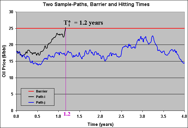
In the chart above, the sample-path "i" reached the aborbing barrier at T*i = 1.2 years, whereas the sample-path "j" didn't reach the barrier level, oscillating below this level during the period of 4 years. This kind of chart can be reproduced by using the spreadsheet simula-hit_time.xls
In this webpage we want to answer questions like:
If the oil prices follow a geometric Brownian motion, what is the expected time for the oil prices to
reach the US$ 25/bbl level? The answer is the mentioned expected first
hitting time for a variable (oil price) that follows a Brownian motion.
Of course the concept is also valid for others stochastic processes.
The mathematical definition for the first hitting time T*(V = b) = T*b for the stochastic process of a value V to reach (or cross) the barrier b, assuming that the process starts with V(t = 0) < b, is given by the equation:

With the standard convention that the infimum of the empty set is infinite.
The barrier b can be the threshold for the optimal investment. In case of perpetual options,
the optimal threshold is a single number (doesn't change along the time), that is, the barrier
is fixed constant.
However, the more general case for options with finite expiration, which
has special practical interest, the threshold for the optimal exercise is
a free-boundary: a term structure of threshold values b(t). We will see later how to estimate E[T*] in both cases.
Recall that the drift (growth rate) is irrelevant to price options when the underlying asset follows a geometric Brownian motion, so that we don't need to especify the drift to find the option value (recall Black & Scholes & Merton model). However, the same is not true for the case of the expected first hitting time calculus. Some options properties like the first hitting time do depend on the drift (the expected growth rate) of the underlying stochastic variable.
In the previous chart with two sample-paths, recall that the path "j" (the blue one) didn't reach the barrier level during 4 years.
The natural question: Is possible that some path never reach the barrier level? In other words, is possible that for one or more sample-paths the time T* = infinite? The answer is: it depends on the drift. If the drift is sufficiently sloped towards the barrier, with probability 1 the sample-paths reach the barrier in a finite time (even being a very long time). However, if the drift is not sufficiently sloped, the problem of sample paths with T* = infinite can happen and the expected first hitting time become a useless concept in this case for practical applications.
The infinite T*, if it happens, is a drawback when using the concept of expected first hitting time. However, it is not a drawback for the next concept: the expected discount factor.
In the option-games applications, is frequently used the expected discount factor, in order to calculate the expected present value of one option that will be exercise at a random time T*.
Imagine that we are interested in this expected discount factor for a stochastic variable X < X* to reach the threshold level X* (when a real option will be exercised). This expected discount factor has a nice closed-form equation:

Note that even if we have many sample-paths with T* = infinite, the exponential values are zeros so that the expectation above there exists (is finite) even with expected first hitting time going to infinite.
In the above equation the parameter "beta1" is the positive root of the quadractic equation from (homogeneous part) option value differential equation (see Dixit & Pindyck, pp.142-144 and p.180). This parameter is function of the stochastic process parameters and the discount rate. We will see that for "real probability" applications, we use the real drift a and the risk-adjusted discount rate r, whereas for "risk-neutral probabilities" applications we replace a by the risk-neutral drift r - d and the risk-adjusted discount rate r by the risk-free discount rate r. See the next topic for a discussion on drifts and discount rates, and see Appendix C for details about the parameter "beta1".
So, if we know the threshold level X* and the option exercise payoff (at X*), we can find out the (perpetual) option value simply by multiplying the exercise payoff by the expected discount factor above.
For a proof of these kind of expectation of a discount factor with random hitting time, click here and see the Appendix B.
Unfortunately, we cannot calculate E[T*] directly from the above closed-form equation. That is:

A frequent mistake is to put the equal signal in the above equation. The time T* is a random variable and in the discount factor equation the random variable T* is inside an exponential function, a convex function. By Jensen's inequality, we cannot calculate E[T*] directly from the above equation.
In reality, due to its convexity and by the Jensen's inequality we can write:

This webpage currently consider the expected first hitting time and expected discount factor only for arithmetic (or ordinary) and geometric Brownian motions. In the future, I intend to extend these concepts to other stochastic processes like mean-reversion and Poisson/jump processes.
The remaining of this webpage is divided as follows. In the next section I discuss the hitting times applications of real versus risk-neutral drifts associated with risk-adjusted and risk-free discount rates, respectively, solving the real options problem using the contingent claims approach. In the third section - the largest one, the formulas for probability density, probability of an eventual absorption, expected first hitting time, and other equations are presented, with discussion and examples for both Arithmetic Brownian Motion and Geometric Brownian Motion, considering a fixed barrier (as in perpetual real options applications). In the fourth section, is showed the case of expected first hitting time for a variable barrier, used in the Excel applicative "Timing". The webpage concludes with the appendixes, including bibliographical references for both the mathematics of first hitting time and real options applications; the proof for the equation of the expected discount rate factor; and an additional discussion about the contingent claims x dynamic programming showing the fundamental quadractic equation for each case.
![]()
The two main applications of the concepts described above are capital planning and valuation of real options and option-games.
In capital planning, projects portfolio managers want to answer the questions:
Assume that a project is not deep-in-the-money with the current market conditions (that is, V < V*).
* When is expected this project to become deep-in-the-money?
* What is the probability of option exercise (investment in the project)?
In real options valuation, contingent claims approach (assume complete markets), we substitute the real drift a by the (unique) risk-neutral drift r - d, which is equivalent to subtract a risk-premium p (> 0) from the real drift a. That is, risk-neutral drift = a - p = r - d.
The figure below illustrates these drifts by showing a real drift and its correspondent (for the same stochastic chocks) risk-neutral drift:
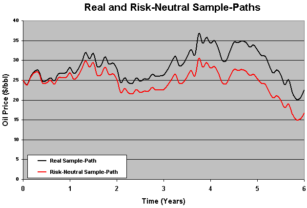
In the above figure, the distance between the sample paths grows at a rate equal to the risk-premium p.
For capital planning problems, is necessary to use the real drift a. The use of risk-neutral drift is a very commom mistake, giving wrong indicators for capital budgeting requirements along the next years (underestimating the required capital) because both the expected first hitting time is overestimated and the probability of option exercise is underestimated.
In risk-management applications such as VaR (Value-at-Risk), is also necessary to work with real drift, not the risk-neutral one.
For options evaluation using risk-neutral drift, the correct discount rate is the risk-free interest rate r. So, for real options valuation, the standard approach is risk-neutral drift + risk-free discount rate.
A less standard approach for real options is by using the dynamic-programming approach (e.g., Dixit & Pindyck) for incomplete markets (martingale measure is not unique and so the RN drift). In this case, even for options valuation, are used the real drift and an exogenous "risk-adjusted" discount rate. For details, see the FAQ Number 4 and the FAQ Number 5.
We are here interested in how to evaluate options using the concept of expected first hitting time and specially the related concept of expected discount factor. Let us see the application of this concept as one alternative to traditional real options optimization under uncertainty problem.
The development below is another way to solve the same optimal investment problem by finding out the expected discount factor from the hitting time T* at the optimal investment threshold V*.
From the expected first hitting time point of view, the general optimal
investment decision problem is modeled as follow:
The firm will wait until the first time T* at which the project value V has reached the optimal level (the threshold) V*, and the firm will then invest.
T* is random variable and depends on the initial level V(t = 0), of the drift, and of the threshold V*.
For the contingent claims approach, the firm will maximize E [ e-
r t] . ( V - I), by choosing
optimally V = V* in order to exercise the option to invest. The optimal exercise of the option occurrs
at t = T*, where T* is the first hitting time of V(t) at the threshold level V*, and I is the investment cost.
For contingent claims approach, we use the risk-free interest rate as discount rate, but in this case is necessary to use the risk-neutral drift r - d for the stochastic process of V(t).
This approach gets the same value obtained for perpetual American call options (e.g., see Dixit & Pindyck, chapter 5).
For the dynamic programming approach, similarly the firm will maximize E [ e- r t] . ( V - I) by choosing optimally V = V* (at t = T*) in order to exercise the option to invest. This case is like the presented in the last paragraph, but for the dynamic programming approach we use r as an exogenous (risk-adjusted) discount rate and the real drift a.
For sample paths which the hitting time T* is infinite, the discount factor is finite: e-
r T* = 0. So, in many situations the expected discount factor is more useful than the expected first hitting time, because the former can exists (be a finite number) even without existing a finite number for the expected first hitting time (if we have some paths with T* = infinite).
In addition, for the GBM, if the drift is higher than 0.5 s2, can be demonstrated that T* is always less than infinite (considering the current V lower than V*), see the end of the next topic.
Let us show how to calculate both threshold and option value for the contingent claims approach. Let the net present value from the option exercise be NPV = V - I.
The maximization of the project is a trade-off between waiting for a higher value of the project V and the discount factor (higher as earlier we exercise the option). If we wait for a too high value of V, we can wait too long time and the discount factor can be too small. So, in this cost-benefit balance of waiting policy, there is one optimal value for V that maximizes the expected payoff from the option exercise , namely the function F (note that F is the real option value!) below:
![]()
Subject to V following a risk-neutral geometric Brownian motion and without constrain in terms of option expiration (the option is perpetual). Let us call the expected discount factor of D(V0, V), where V0 is the initial value of the stochastic variable V0 = V(t = 0).
So, our function F becomes:
F = Max D(V0, V) . ( V - I)
The first order condition to maximize the above equation determines that we take the partial derivative of F in relation to the stochastic control variable V, and equaling to zero. We obtain:
D(V0, V*) + DV*(V0, V*) . V* = DV*(V0, V*) . I
Where DV*(V0, V*) is the partial derivative of D in relation to V (or V* at the optimum V = V*). This derivative is easily calculated because we know that (see the Introduction and the proof in the Appendix B):

Hence, the derivative DV*(V0, V*) is:

Now, simply substitute D(V0, V*) and DV*(V0, V*) in the equation that we found with the first order condition and after a few algebra steps:

This is a well known equation: the threshold is the "wedge" (> 1) times the investment.
Now, we can find easily the real option value F by substituing the threshold in the equation F = E [ e- r t] . ( V* - I). That is:
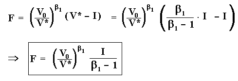
Case with two correlated geometric Brownian motions: In a more general setting, the investment cost can also follow a GBM, which can be correlated with the GBM for the completed project value V.
In this case, thanks to the first degree homogeneity of the option value in relation to V and I and thanks to zero degree homogeneity for the threshold (e.g., see McDonald & Siegel, 1986), we
can work with the ratio p = V/I, and so the threshold will be a ratio p* = (V/I)*, and with a compound "total volatility".
This threshold ratio p* and the normalized real option value f = F / I, can be found with the same approach.
![]()
In this section is examined the case of hitting time to a constant barrier. This case occurrs tipically for perpetual real options, which the threshold for optimal investment is a constant value (independent of time). However, another important case is the possibility of one asset to drop until the value zero, as in bankruptcy.
Next, is presented the case of an absorbing barrier at zero for Arithmetic Brownian Motion. After that, the extension to the non-zero barrier case, and finally the extension for the Geometric Brownian Motion.
The Arithmetic Brownian Motion, with drift a, starting at V0 in t0, is given by:
dV = a dt + s dz
We are interested in the first hitting time that the stochastic variable V(t) reaches (or crosses) one fixed barrier b. Let us see the case of barrier at zero.
A problem of practical importance is the possibility of an asset
(security, firm value, project value, etc.) value dropping to zero where
remains forever (zero as absorbing barrier).
For example, if a stock of one firm drops to zero, the firm is in bankrupt and the stock value remais forever at zero.
One approach to model this issue is by using a Poisson process with a discrete jump down to zero ("sudden
death").
However, for the case of a continuous stochastic process, e.g., following
a Brownian motion, we need to use the concepts of first hitting time and
absorbing barrier.
Formally, at absorbing barrier V = 0 the stochastic process for V is over,
meaning that V remains at 0 forever. For the Geometric Brownian Motion this is endogenously true, because if V = 0 then
dV = 0, because dV = a V dt + s V dz.
For the Arithmetic Brownian Motion, we can set an absorbing barrier at 0 (or other value), saying that something happen at this barrier,
such as the firm bankrupt or some option is exercised, stopping the (interest on the) stochastic process for that application.
The solution for these kind of problems, where we need to know the probability distribution and/or probability moments (like mean and variance), generally is solved using the Kolmogorov equations. The Kolmogorov forward equation, also called Fokker-Planck equation, given the initial conditions, the current state V0 and the current time t0, we obtain the transition probability to future state V1 and t1, by working with derivatives of the future state.
The Kolmogorov backward equation, which is very similar to the Black-Scholes equation, works with derivatives of the current state V0 and t0.
In this section, I don't develop these equations: I put directly the results. However, interested readers can consult the following books: Dixit & Pindyck (1994, appendix chapter 3); Dixit ("The Art of Smooth Pasting", 1993); Ingersoll (1987, "Theory of Financial Decision Making"); or Willmott ("Paul Wilmott on Quantitative Finance", 2000, vol. 1, chapter 10).
Following Ingersoll's textbook (1987, pp.353-354) but with our notation, the first hitting time probability density function g(t; V0, t0) to reach the absorbing barrier V = 0 (conditional to V starting at higher value) is given by:

Where n(.) is the standard normal probability density.
Using the known equation for n(.) and setting t0 = 0, the
density g(t; V0) equation can be written:

The probability density chart for the first hitting time that V, starting from V0, reaches the absorbing barrier V = 0, is illustrated below for two volatilities cases:
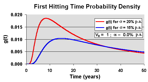
The chart above shows that higher volatilities means early hitting time (or higher probability density for smaller passage times). This is very intuitive.
What if the barrier b is placed above the current level, that is, b > V0 ?
The probability density is given by Karlim & Taylor (A First Course in Stochastic Processes, 2nd edition, p.363) or by Cox & Miller (The Theory of Stochastic Processes, p.221, eq.74, for the case of V0 = 0):

Compared with previous equations, there is a translation with V0 being replaced by b - V0, the (modulus) of the distance up to the barrier (recall that probability density function never is negative). There is also an adjustment in the drift signal because in this case the drift has an opposite effect, when compared with the case of a barrier placed below the current level (at zero, in the previous equations).
For the driftless case, a = 0, in the above density equation, T has no finite moments (Cox & Miller, p.221). We will discuss later the first moment case (expected first hitting time).
The (cumulative) probability distribution of hitting times for the above case is given by the equation below. This equation is 1 less the probability of not hitting given by Harrison (Brownian Motion and Stochastic Flow Systems, p.14, eq.11):
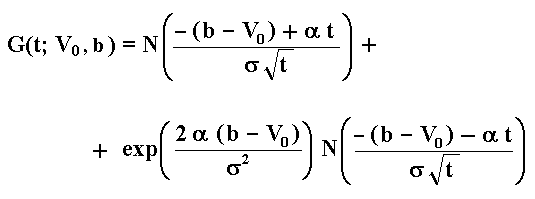
Where N(.) is the standard Normal (cumulative) probability distribution.
The reader can check that this distribution increases with both the drift and the volatility.
The equations above are for the arithmetic Brownian motion. Later, we will see that, by using these expressions, is very easy to derive the equivalent expressions for geometric Brownian motion, with a logarithm transformation and with change in the drift. Anyway, both the probability density and the cumulative probability distribution for the geometric Brownian case are showed in the Excel spreadsheet placed at this webpage.
The probability to occur an eventual absorption at the absorbing barrier placed at V = 0, is:
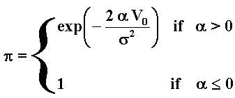
So, if the drift is negative or zero, almost surely (with
probability 1) the process will reach zero in a finite time.
This probability is important for the classical gambler's ruin problem. It shows that even for a fair game (drift = 0), almost surely one day he/she will lose all the money, if he/she never stops. This probability is also important for financial applications such as the credit risk (default probability) and problems of economic survival in general.
For positive drift, the probability of V to hit the zero level is
increasing with volatility and decreasing with the initial level V0
and with the drift.
In others words, for positive drift there is a probability (
1 - p ) of the zero level never to be reached
(or hitting time equal infinite with probability [1 -
p] for positive drift).
However, the probability of some day the stochastic process reach/cross
the zero value can be very small. Examples:
(a) for V0 = 10; a = 2% p.a.; and
s = 20% p.a., we get p
= 0.0045% (~zero);
(b) in the same case but with a = 0.5 %p.a.;
the probability increase to p = 8.21%;
(c) if V0 = ln(10) = 2.3026; a =
2% p.a.; and s = 20% p.a., we get
p = 10%.
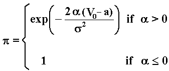
What is the probability of an eventual absorption if instead zero the barrier is placed at positive level, but below the current value V0. The probability of an eventual absorption if the barrier "a" is so that 0 < a < V0 is given by the equation 6.5 from the Dixit's book "The Art of Smooth Pasting", which is just the previous equation with a translation, that is, replacing V0 by the (modulus) of the distance V0 - a in the previous equation.
So, the probability of an eventual absorption for a positive barrier a < V0 is:
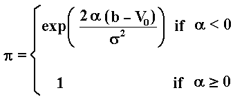
What if the barrier is placed above the current level V0? The expression below, the probability of an eventual absorption for a barrier b > V0, can be found in Cox & Miller (p.212, eq.39):
Now imagine two barriers, a lower barrier "a" and a upper barrier "b". What is the probability that the first barrier hit is "a", not "b"? The answer is given by the same Dixit's book (equation 6.4):
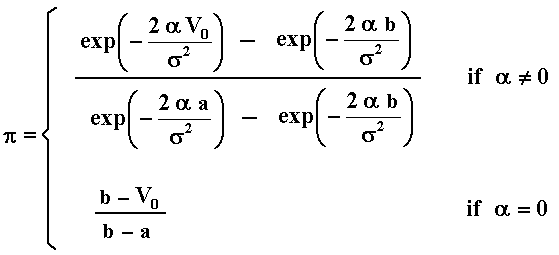
Where the second line (for driftless processes) is obtained with the limit when the drift tends to zero from the first line equation. Similarly, the probability that the first barrier hit is "a", not "b" is simply 1 - p
Hence, there is zero probability that this process evolves between the two barrier without ever hitting either (see Dixit, p.54), even for driftless processes.
The equations above are valid for arithmetic Brownian motion. The extension to geometric Brownian motion is straightforward by using a logarithm transformation that we will see soon. Before it, let us see the expected first hitting time for the arithmetic Brownian motion.
For this problem (arithmetic Brownian, only one absorbing barrier at zero), Ingersoll's textbook (Theory of Financial Decision Making, 1987, p.354, eq.41) presents the expected first hitting time equation:
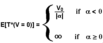
Ingersoll points out two alternative demonstrations for these equations.
The first one is by taking the distribution of the V stochastic process
(eq. 31, p.352 in his textbook, derived from Kolmogorov differential
equation) and relating with the distribution of hitting time (eq.33, p.353
in his textbook). The second way is by using the Kolmogorov backward
differential equation directly for the hitting time distribution (and
density) with appropriate boundary conditions. In this case is used the
Laplace transformation of g.
Although the above equation is a classical result, it is something surprising the independence of the volatility in the expected first hitting time above. However, we will see that for the geometric Brownian motion, the expected first hitting time will depend on volatility.
Even with negative drift, the expected hitting time can be very long if
the current value is sufficiently far from the zero level barrier. For
example:
(a) V0 = 10 and a = - 2% p.a., we
get E[T*(V = 0)] = 500 years; and
(b) V0 = ln(10) = 2.3026 and a = -
2% p.a., we get E[T*(V = 0)] = 115 years.
Lets expand the Ingersoll's hitting time formula presented above, for the
case of a lower but nonzero absorbing barrier a, where 0 < a <
V0.
This case is important in real options applications, for example to know
the expected exit time for a firm facing a declining demand for a
quasi-obsolete product (e.g.: product with life cycle, as in computer
industry), where "a" is the abandon threshold.
The difference from the E[T*(V = 0)] equation is very small: if instead E[T*(V = 0)] we want E[T*(V = a)], it is only a translation. So, just replace V0 for (V0 - a) (see Dixit's The Art of Smooth Pasting, p.56, eq.6.10).
Hence, for the barrier a < V0, the first hitting time for arithmetic Brownian motion is:
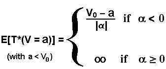
An equivalent expression is presented in Dixit's book (The Art of Smooth Pasting, p.56, eq.6.10).
Ross (Stochastic Processes, 2nd edition, p.364) after showing the infinite expectation for the driftless case, wrote about the first hitting time T*: "though finite with probability 1, has an infinite expectation. That is, with probability 1, the Brownian motion process will eventually hit a, but its mean time is infinite".
Prof. Dixit give us an explanation about E[T*] = infinite for driftless process (a = 0):
"...the probability of an eventual hit is unity. But very long excursions away from the barrier can occurr. Then the probabilities do not fall sufficiently fast for successively longer hitting times, and the expectation, which is the sum of the products of the times and their probabilities, divergers."
In the same book Prof. Dixit teaches at p.55: "... some events may have infinite expected time, either because there is a positive probability that they never happen, or because probabilities of very long delays decrease too slowly."
For applications of investment option exercise, in general the barrier (threshold) is placed above the current level V0. The changes in the above equation are few and ease to understand. So, for the barrier b > V0, the first hitting time for arithmetic Brownian motion is:
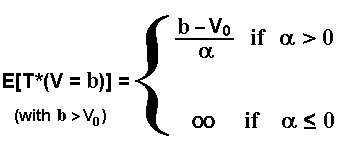
If the drift is positive, the variance of the first hitting time is also finite. The variance depends on the volatility and for the above case, b > V0, the variance is given by:

This result can be found in Cox & Miller (p.222, eq.76 for V0 = 0) . More general closed-form results on expected first hitting time and variance of hitting times for arithmetic Brownian motion can be found in Dominé, M. (1995): "Moments of the First Passage Time of a Wiener Process with Drift Between Two Elastic Barriers", Journal of Applied Probability, Vol.32, 1995, pp.1007-1013 (however, there is a typo in the variance equation, p.1013).
Somebody can ask about the utility of arithmetic rather geometric
Brownian process for real options applications. The point is that
sometimes is useful to see the Geometric Brownian motion as an Arithmetic Brownian for the logarithm of the project value.
Following Dixit's textbook The Art of Smooth Pasting (p.7):
if dV/V = a dt + s
dz, letting v = ln(V), and using Itô's Lemma we find that v
follows the arithmetic (or ordinary) Brownian motion:
dv = d(lnV) = (a - ½
s2) dt + s
dz
so,
dv = a' dt + s dz
Although the volatility term is the same, as highlighted by Dixit, d(lnV)
is different of dV/V - in reality, by the Jensen's inequality, d(lnV) <
dV/V.
There is a frequent confusion between d(lnV) and dV/V (people saying that
is the same thing). Sometimes this confusion has no practical importance
because the drift value doesn't matter for several applications (the case
of many options calculations, like the Black & Scholes famous
equation), but this is not the case here. As discussed before, for the
hitting time calculations, the drift a
matters, and there is a difference of ½ s2
dt between these processes.
Given this alert, due to its simplicity could be interesting to work with logarithm diffusion equation, so using arithmetic Brownian motion, easing the calculus in Kolmogorov equations (calculus of probabilistic moments) or easing Monte Carlo simulations.
With the insights above and given that we have the results for the arithmetic Brownian case, we can easily find out the expected first hitting time equation for the Geometric Brownian Motion. As before, let us divide the analysis into two cases. First, the barrier (or boundary) V* is below the current value for the stochastic variable, that is, for the case with a < V0 (e.g., abandon threshold), the expected first hitting time if V follows a GBM is:

This kind of equation also appeared in the book of Willmott & Dewynne & Howison (1993, p.371, eq.B3).
For applications of investment option exercise, in general the barrier (threshold) is placed above the current level V0. The changes in the above equation are few and ease to understand. So, for the barrier b > V0, the first hitting time for geometric Brownian motion is:

Numerical example for the first equation (a < V0):
Assume that V = 10, s = 25%pa, a = - 20%pa. (drift of dV/V), and the exit
threshold is V* = 8.
What is the expected exit time for the firm?
Solution:
a' = - 0.2
- ½ 0.252 =
- 26.25%pa.
So, E[T*(V = 8)] = ln(10/8)/0.2625
So, E[T*(V = 8)] = 0.85 years (or 10 months).
See the difference between expected first hitting time and expected
value of V in t = 0.85 years.
E[V(t = 0.85)] = V0 ea Dt
= 10 exp(-0.2 x 0.85) = 8.44 > V* = 8.
In reality, only at about t = 1.1 years, the expected value of V is V* =
8. Formally, E[V(t = 1.1)] = V* = 8.
So, expected first hitting time to reach a certain level is not equal to
the time that V is expected to be a certain level.
In a V x t chart, one expected value is calculated in the horizontal
(expected first hitting time) and the other one is calculated in the
vertical (expected value of V).
What happens if instead a volatility of 25%pa, this parameter increase
to 40%?
The reader can see that the expected first hitting time E[T*] decreases,
whereas it has no effect on the expected future value of V, that is, there
is no effect on E[V(t)].
Now, imagine that one firm plan to expand the production (exercising one option to invest) if the demand rises to a certain level V**, but if the demand drops to the (nonzero) level V*, the firm will abandon the business. What is the expected first hitting time for either thresholds? In other words, what is the expected time for V to exit the region between V* and V**?
The solution is given by Willmott ("Paul Wilmott on Quantitative Finance", 2000, vol. 1, p.163):

Where V0 is the initial value for the stochastic variable, V(t = 0).
Now, I discuss some issues related to the above equation, not discussed in the Willmott's book:
- For V* = 0, in the above equation we need to obtain the limit when V* tends to zero. The resulting expression is left as exercise for the reader (tip: there exists the limit except when a = 0.5 s2).
- What happens with E[T*] if a = 0.5 s2 (assuming V* > 0)? Is E[T*] = infinite? Can the value be obtained by taking the limit when a tends to 0.5 s2?
The answer is: this equation converges to a finite time (recall the discussion on probability of eventual absorption). The reader can also verify numerically the convergence by using the spreadsheet simula-hit_time.xls and letting a' very near 0.5 s2. Or, by using the analytical limit expression given by:

However, when both V* tends to zero and a tends to 0.5 s2, we have E[T*] = infinite.
Why? Tip: recall the Dixit's discussion (The Art of Smooth Pasting, p.56) just after his eq.6.10 (or see our quotation above).
The spreadsheet below illustrates many formulas above for fixed barrier(s) and generates sample-paths for both fixed and variable barrier. This spreadsheet is freeware for educational purposes (hope mentioning the source when using it).
![]() Download the Excel for Windows file
simula-hit_time.xls, with 190 KB.
Download the Excel for Windows file
simula-hit_time.xls, with 190 KB.
The spreadsheet above consider the oil prices P following a geometric Brownian motion (GBM), presenting charts and formulas, including some equations not showed explicitly before (GBM case):
* hitting time probability density for the GBM case;
* hitting time cumulative probability for the GBM case
* probability of eventual absorption for one and two barriers for the GBM case, etc.
![]()
The discussion and the equations above are elegant and relatively simple. However, these methods are useful for perpetual options and related applications with a fixed barrier, not for finite lived options where we have a variable barrier b(t). In mathematical jargon, b(t) is a free boundary representing the threshold curve for optimal option exercise for finite lived options.
At the best of my knowledge, there is no analytical/closed-form equations for both expected first hitting time and expected discount rate, when the barrier is a free-boundary. There are some analytical methods for barriers b(t) with some specific (and simple) function of the time, but not for this kind of free-boundary that cannot be described with a simple function.
However, numerical methods are available to solve this problem. One alternative is to solve numerically the Kolmogorov differential equation. However, I use the Monte Carlo method in order to get both expected first hitting time and probability of option exercise because it is much simpler considering that I get the free-boundary before the simulation.
In cases with negative drift and in cases with finite time to expiration, we can think to get both prob[exercise] and E[T*|exercise], respectively the probability of exercise and the expected first hitting time conditional to the option exercise occurrence. With these two informations we can caracterize the stochastic problem, providing important information on the future investments schedule, helping the capital budget planning.
Here we are interested only in capital planning problems, because the use of these concepts to solve the option pricing problem is not competitive with others methods (including analytical approximations available in the literature) for finite-lived American options.
Hence, I use the real drift a not the risk-neutral drift (recall the discussion in the second section of this webpage).
The picture below illustrates how to estimate the conditional expected hitting time and the probability of option exercise using the Monte Carlo approach. The picture shows the free-boundary (threshold curve for optimal option exercise) and two sample paths from Brownian motion. The black path reaches the free-boundary line (point A) before the expiration, whereas the blue sample path doesn't reach the free-boundary during the option life.
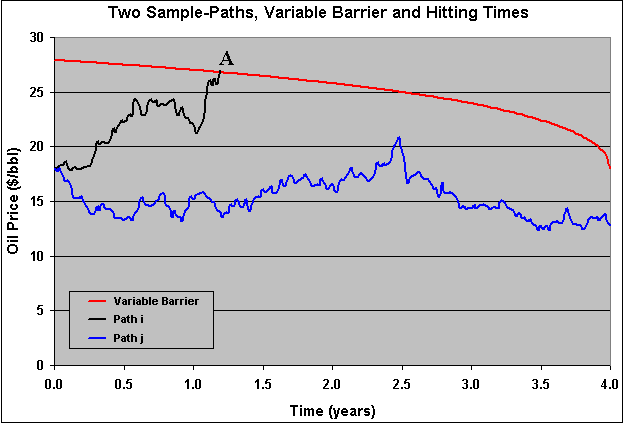
This kind of chart can be reproduced by using the spreadsheet simula-hit_time.xls
Timing version 2.0 calculates the expected probability of
exercise using (Quasi) Monte Carlo Simulation. This probability is
simply the number of paths that hit the threshold line divided by the
total number of sample paths simulated.
In order to download the full functional shareware Timing, click here.
In order to know more about this applicative, go to Timing webpage.
Timing version 2.0 also calculates the expected time of option exercise, conditional to the option exercise occurrence. This expected first hitting time here is calculated only for the sample paths that hit the threshold line and it is the average time of hitting the threshold line for these winner sample paths.
Timing version 2.0 calculates the optimization problem before and separated of the T* calculus. In other words, the free-boundary V*(t) is an input for T* calculation and so is calculated before.
The software Timing version 2.0 calculates the conditional expected first hitting time and the probability of the option to be exercised, for finite lived options, using the Monte Carlo approach. The figure below illustrates these facilities in the software "Timing":
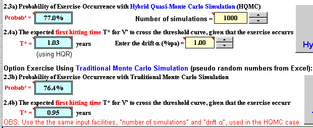
In the above figure we see that there are two alternatives to calculate the conditional expected hitting time and the probability of exercise. The first alternative is by using the more precise hybrid quasi-random numbers, see the webpage on the quasi-Monte Carlo and the section with hybrid quasi-random sample-paths. The second one is by using the traditional pseudo-random numbers (from Excel).
Note also in the above figure that is required the drift in order to calculate both the expected first hitting time and the probability of option exercise. Recall from previous sections that, although in option pricing generally we don't need to know the drift, this is not valid for the case of the expected first hitting time calculus. Some options properties like the first hitting time do depend on the drift (expected growth rate) of the underlying stochastic variable. So, in this Excel application you need to set the drift.
In the last picture, at the extreme right side the simulation buttons are cut. The figure below shows the two buttons, one for quasi-Monte Carlo simulation and the other for the traditional Monte Carlo simulation.
![]()
The results of expected first hitting time, probability distribution of hitting times, and Kolmogorov equations applied to Brownian motion, the reader can find further informations in the following books:
Dixit & Pindyck (1994, appendix chapter 3); Dixit ("The Art of Smooth Pasting", 1993); Ingersoll (1987, "Theory of Financial Decision Making"); or Willmott ("Paul Wilmott on Quantitative Finance", 2000, vol. 1, chapter 10).
Dixit uses the discrete-time random walk approach to find results in continuous-time with limiting arguments. Hence, this more intuitive approach can be preferable for beginners in this field.
At the best of my knowledge, the earliest application of optimum option
exercise using the concept of first hitting time, is due to Karlin and
Taylor (1975) textbook, A First Course in Stochastic Processes
(pp. 363-365), which the authors find both the threshold and the option
value. Their demonstration using hitting time
probability density and Laplace transformation, is different of the
mentioned Dixit & Pindyck book (1994, appendix, chapter 9) way,
presented here in the Appendix B. Alternative ways providing the same
results bring more reliability for the results!
This approach is best explained in the Dixit & Pindyck & Sodal (1997) working paper (published by Economic Journal, April 1999, pp. 179-189), which develops an alternative way to find the
optimal V*, based in the Baily's Ph.D. dissertation, MIT 1995.
See also a more recent paper of Sodal: "Entry, Exit and Scrapping Decisions with Investment Lags: A Series of Investment Models Based on a New Approach",
presented at the 5th Annual International Conference on Real Options, UCLA, July 2001.
For perpetual options and in general for problems with a constant barrier, this way to solve the investment under uncertainty problem is very promising.
For the reader interested to go further in mathematical theory of first hitting time, there are methods
like presented by Karatzas and Shreve (see in their book, second
edition, the topics in pp. 2, 79, 94, and 196, the last one for Brownian motion with
drift) using Laplace transforms and mathematical concepts like the reflection
principle and martingales (considerations based on the optimal
sampling theorem for martingales).
OBS: the reader shall pay attention in mathematical texts like that, because most results are for a "standard" Brownian motion that is an Arithmetic Brownian motion with volatility equal 1. Although the mathematicians consider the extension to a non-unity volatility as a "straightforward rescaling", formulas assuming volatility equal one is useless for financial economics practice (unless the user is also a specialized mathematician).
Other very important source (and perhaps easier) for hitting time is the
Harrison's textbook. See his warning about the use of "reflection
principle" - valid only for simmetrical or driftless processes, in the introduction and general theory in pp.7-14 and
pp.38-42. The book presents an useful focus on expected discounted costs
(see paragraph 2, p.38, specially p.39, and pp.44-49).
In addition, although many proofs are performed for the case of unity volatility (s = 1), he presents the general results for any volatility value s > 0.
Another excellent source (and also easier than Karatzas and Shreve) is the
book of Karlin & Taylor (1975), A First Course in
Stochastic Processes, second edition.
See for example the theorem 5.2 (p.361) for the probability that the
process reaches the level b (above the initial level) before hitting the
level a (below the initial level).
The most interesting case is the optimization problem for a perpetual
option: they show how to compute the threshold (early exercise level)
using the concept of expected first hitting time (see pp.363-365).
A classical textbook that remains as a valuable reference is Cox & Miller (1965), The Theory of Stochastic Processes. See the chapter 5 for proofs of some equations presented in this webpage.
Why the expected first hitting time is useful in real options? Let us answer with some examples (consulte the bibliographical list webpage for the complete reference):
Suppose an expected discount factor in continuous time, with a generic (exogenous) discount rate r:
f(V) = E[e- r t]
Denoting the first hitting time as T* (first time that V is equal or larger than V*), here representing when the option to invest will be optimally exercised, the expected discounted payoff from T* to current date is exactly the current value of the option to invest. Assuming that the current V < V* and by choosing an interval dt sufficiently small that hitting the threshold V* in the next short time interval dt is an unlike event, the problem restarts from a new level (V + dV). Therefore we have the dynamic programing-like recursion expression:
f (V) = e- r dt E [ f (V + dV) | V] = e- r dt { f(V) + E [ df(V) ] }
By noting that:
(a) V follows a geometric Brownian motion with drift a
and volatility s; and
(b) Using the Itô's Lemma for expanding df (V), and using the
subscripts to denote derivatives we have:
df = fV (a V dt + s V dz) + 0.5 fVV (s2 V2 dt) = fV a V dt + fV s V dz + 0.5 fVV s2 V2 dt
Note that we are supposing the infinite time horizon (perpetual option)
case so that the variable time is not included in the Itô's Lemma.
By substituing df into the previous equation and by noting that E[dz] = 0,
and letting e- r dt = 1
- rdt for a very small dt, we get:
f (V) = (1 - rdt) { f + fV a V dt + 0.5 fVV s2 V2 dt }
With a few algebra (remember dt2 is zero) the reader can find out the following differential equation:
1/2 s2 V2 fVV + a V fV - r f = 0
Where the subscripts denote derivatives. The general solution is:
f (V) = A1 Vb1 + A2 Vb2
Where b1 and b2 are the respectively the positive and the negative roots of the standard quadratic characteristic equation from the differential equation (see an instructive discussion of the characteristic equation in chapter 5, section 2.A, of Dixit & Pindyck book).
Applying two boundary conditions: as V approximates to the threshold V*,
T* is probable to be small and the discount factor f(V) close to 1, so
f(V*) = 1. When V is close to zero, T* is likely to be large and so the
discounted factor close to zero, therefore f(0) = 0 (note: alternatively,
I think is possible to see V = 0 as an absorbing barrier, so when V tends
to zero, T* tends to infinite or there is no finite time for V to reach
the threshold from V = 0).
With these results, we can see that A1 = (1/V*)b1
and A2 = 0.
Therefore the solution for the expected discount factor is:
Where V is the initial value of the stochastic variable, that is, at t = 0. So the expected first hitting time is estimated by assuming that T* is finite. The parameter b1 is given by the equation (positive root of the fundamental quadratic equation, see the quadratic equation and a discussion at the end of the next appendix):

The case of contingent claims is similar, by substituing the discount rate r by the risk-free interest rate r and by replacing the real drift a by the risk-neutral drift r - d. See more details about contingent claims x dynamic programming in Appendix C.
For an application of these kind of hitting time expectation, see the leader value in symmetric duopoly under uncertainty.
A similar demonstration of these kind of expectations for option-games can be found here.
For an even more general approach (for any stochastic process) and a more detailed discussion using hitting time, see the working paper of Dixit & Pindyck & Sodal (1997).
The two most used approaches for dynamic optimization under uncertainty
are Bellman's equation (dynamic programming under uncertainty) and
contingent claims. It is true that there exist also the Lagrangian method developed by G. Chow
and the hitting time approach (Dixit & Pindyck & Sodal) discussed above which the following
discussion is useful.
For each method the drift and discount rates have special features which
is discussed briefly in this appendix.
In situations where is reasonable to assume the market as sufficiently complete is preferable to use contingent claims approach and in this case the general PDE (partial differential equation) for several real options problems is:
0.5 s2 V2 FVV + ( r - d ) V FV - r F = - Ft
Where F is the option, V is the project value (the underlying asset),
and the subscripts denote partial derivatives.
This is also the Black-Scholes PDE (call or put, depending on the boundary
conditions) for the case of stock with dividend yield.
Now, if we don't know if the market is complete, people can use the
Bellman's equation (dynamic programming under uncertainty), assuming an
exogenous discount rate r and the PDE for
several real options problems is:
0.5 s2 V2 FVV + a V FV - r F = - Ft
The equivalence:
if the market is sufficiently complete to be priced by arbitrage (so there
exists an unique equivalent martingale measure) you can substitute the
drift into the last PDE: a = r
- d AND substitute r
= r.
The first and the second PDE are equal with that substitution.
In others words, by changing the drift is possible to use the risk-neutral
valuation.
See Dixit & Pindyck book (1994, chapter 4, the comment of eq.20), which the authors explain the equivalence of these two approaches for geometric Brownian case. For a further general discussion about the equivalence between the two approaches for real options, see the same book, chapter 4, section 3.
We use one specific case of the PDE for the hitting time problem: the
perpetual option case. In this case the derivative of option in
relation to the time is zero ( Ft = 0 ).
The perpetual option has an analytical solution that needs to know the roots from the fundamental quadratic equation from the differential equation.
In general only the positive root is required, but in hysteresis model and other models with entry and exit options, are necessary both positive and negative roots. This quadratic equation, for the standard dynamic programming approach with geometric Brownian motion, is given by:
0.5 s2 b ( b - 1 ) + a b - r = 0
With r > a.
The positive (and > 1) root solution is:

If instead the parameter that you know is d, set the drift a = r - d, and the fundamental quadratic is:
0.5 s2 b ( b - 1 ) + ( r - d ) b - r = 0
For complete market/contingent claims approach, the fundamental quadratic (characteristic) equation is the above equations but setting a = r - d AND substitute r = r, so the quadratic equation becomes:
0.5 s2 b ( b - 1 ) + ( r - d ) b - r = 0
![]()
![]()